뉴욕시의 총 택시 운행 기간 예측
In this competition, Kaggle is challenging you to build a model that predicts the total ride duration of taxi trips in New York City.
Your primary dataset is one released by the NYC Taxi and Limousine Commission, which includes pickup time, geo-coordinates, number of passengers, and several other variables.
- id - a unique identifier for each trip
- vendor_id - a code indicating the provider associated with the trip record
- pickup_datetime - date and time when the meter was engaged
- dropoff_datetime - date and time when the meter was disengaged
- passenger_count - the number of passengers in the vehicle (driver entered value)
- pickup_longitude - the longitude where the meter was engaged
- pickup_latitude - the latitude where the meter was engaged
- dropoff_longitude - the longitude where the meter was disengaged
- dropoff_latitude - the latitude where the meter was disengaged
- store_and_fwd_flag - This flag indicates whether the trip record was held in vehicle memory before sending to the vendor because the - vehicle did not have a connection to the server - Y=store and forward; N=not a store and forward trip
- trip_duration - duration of the trip in seconds (target)
import pandas as pd
import matplotlib.pyplot as plt
import seaborn as sns
import numpy as np
import warnings
from datetime import datetime
import calendar
from math import sin, cos, sqrt, atan2, radians
from folium import FeatureGroup, LayerControl, Map, Marker
from folium.plugins import HeatMap
import matplotlib.dates as mdates
import matplotlib as mpl
from datetime import timedelta
import datetime as dt
warnings.filterwarnings('ignore')
pd.set_option('display.max_colwidth', -1)
plt.style.use('fivethirtyeight')
import folium
from sklearn.cluster import KMeans
from sklearn import preprocessing
from sklearn.model_selection import train_test_split
from sklearn.impute import SimpleImputer
from sklearn import linear_model
from sklearn.metrics import mean_squared_error
from sklearn.ensemble import RandomForestRegressor
import pickle- Imputer 함수 사용 불가 (업데이트 ; 코드에러) => from sklearn.impute import SimpleImputer 로 해결
train=pd.read_csv("C://Input/train.csv")
test=pd.read_csv("C://Input/test.csv")
test.shape
train.info()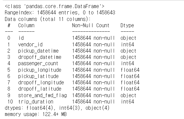
- 'pickup_datetime' , 'dropoff_datetime' 의 Dtype이 object 이다.
Convert to appropriate datatype - 날짜 데이터 형식 변경
convert pickup dateime and dropoff datetime into date-time object
to_datetime() : 판다스를 이용한 데이터 타입 변환중 날짜에 관한 함수
- datetime64형식으로 변환 하는 방법날짜 변수를 datetime64형식 으로 데이터 타입 변경하기
train['pickup_datetime']=pd.to_datetime(train['pickup_datetime'],format='%Y-%m-%d %H:%M:%S')
train['dropoff_datetime']=pd.to_datetime(train['dropoff_datetime'],format='%Y-%m-%d %H:%M:%S')
train.head()
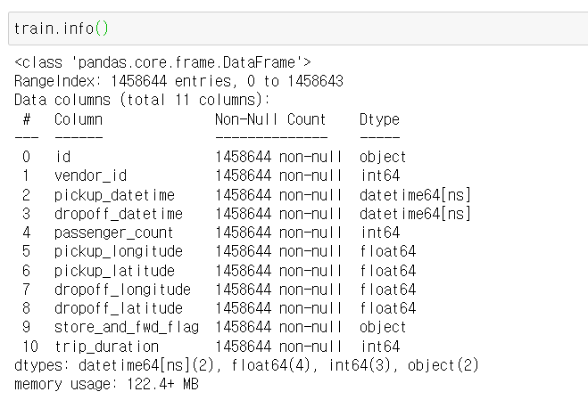
- 'pickup_datetime' , 'dropoff_datetime' 의 Dtype이 datetime64[ns] 이다.
→ 데이터 타입 변경 완료 !
Are there any missing values in the data ? - 결측치가 있는가 ?
train[pd.isnull(train)].sum()
- There are no missing values
What is the time period of the dataset? - 데이터 수집 기간
print("Min pickup time:",min(train['pickup_datetime']))
print("Max pickup time:",max(train['pickup_datetime']))
Min pickup time: 2016-01-01 00:00:17
Max pickup time: 2016-06-30 23:59:39
- The data has 6 months of taxi trip data, from Jan to Jun 2016
create new day,month, hour info from Pickup time - 날짜, 시간, 요일 변수 생성
train['pickup_date']= train['pickup_datetime'].dt.date
train['pickup_day']=train['pickup_datetime'].apply(lambda x:x.day)
train['pickup_hour']=train['pickup_datetime'].apply(lambda x:x.hour)
train['pickup_day_of_week']=train['pickup_datetime'].apply(lambda x:calendar.day_name[x.weekday()])
train['dropoff_date']= train['dropoff_datetime'].dt.date
train['dropoff_day']=train['dropoff_datetime'].apply(lambda x:x.day)
train['dropoff_hour']=train['dropoff_datetime'].apply(lambda x:x.hour)
train['dropoff_day_of_week']=train['dropoff_datetime'].apply(lambda x:calendar.day_name[x.weekday()])
- 'pickup_day' : 택시를 탄 날짜 (일)
- 'pickup_hour' : 택시를 탄 시각 (시간)
- 'pickup_day_of_week' : 택시를 탄 요일
Round lat lng to 3 decimal places - 소수 셋 째 자리에서 반올림
train['pickup_latitude_round3']=train['pickup_latitude'].apply(lambda x:round(x,3))
train['pickup_longitude_round3']=train['pickup_longitude'].apply(lambda x:round(x,3))
train['dropoff_latitude_round3']=train['dropoff_latitude'].apply(lambda x:round(x,3))
train['dropoff_longitude_round3']=train['dropoff_longitude'].apply(lambda x:round(x,3))

train.head()
Based on Latitude and Longitude get the distance of the trip in km - 주행거리
- 위도 및 경도에 따라 주행 거리(km) 구하기
- This uses Haversine Distance
Haversine 거리 :
https://towardsdatascience.com/spatial-distance-and-machine-learning-2cab72fc6284

- radians : 각도 x를 라디안으로 변경해주는 함수
- axis=1 : 가로 방향으로 연산 ( 한 행의 모든 열에 대하여 연산 )
- 주행 거리
def calculateDistance(row):
    R=6373.0 # approximate radius of earth in km
    pickup_lat=radians(row['pickup_latitude'])
    pickup_lon=radians(row['pickup_longitude'])
    dropoff_lat=radians(row['dropoff_latitude'])
    dropoff_lon=radians(row['dropoff_longitude'])
    dlon = dropoff_lon - pickup_lon
    dlat = dropoff_lat - pickup_lat
    a = sin(dlat / 2)**2 + cos(pickup_lat) * cos(dropoff_lat) * sin(dlon / 2)**2
    c = 2 * atan2(sqrt(a), sqrt(1 - a))
    distance = R * c
    return distance
train['trip_distance']=train.apply(lambda row:calculateDistance(row),axis=1)
train.head()
- 주행 시간 (시간)
train['trip_duration_in_hour']=train['trip_duration'].apply(lambda x:x/3600)
train.head()
Q. 3600으로 나눠주는 이유 ?
- trip_duration - duration of the trip in seconds / 여행기간 (초)
- 초를 시간으로 나타내기 : 60 * 60 = 3600
Exploratory Analysis
- 'trip_duration_in_hour' 변수 그래프
plt.figure(figsize=(8,5))
sns.distplot(train['trip_duration_in_hour']).set_title("Distribution of Trip Duration")
plt.xlabel("Trip Duration (in hour)")
- There are trip duration greater than 24 hours. We will have to investigate this?
- 여행시간이 24시간이 넘어가는 경우 추출
outlier_trip_duration=train.loc[train['trip_duration_in_hour']>24]
outlier_trip_duration
There are 4 records which have very high trip duration, but the distance travelled is very low. These are outliers.
But is there any particular location to which these trips begin or end?
Trip duration is also skewed, so let us take log transformation.
We will not remove these from the analysis, because they might be a part of test data as well

→ 주행 시간은 24 시간이 넘어가지만 주행 거리는 매우 짧다.
* 주행 기간이 매우 긴 기록이 4개 있지만 주행 거리는 매우 낮습니다. 이들은 특이치입니다.
하지만 이 여행이 시작되거나 끝나는 특별한 장소가 있는가? 주행 기간 또한 왜도가 크다.
로그 변환을 수행하겠다.
또한 테스트 데이터의 일부일 수 있으므로 분석에서 이를 제거하지 않습니다.
- 'trip_duration' 에 로그를 취한다. ; 'Trip duration' 는 왜도가 있으므로
plt.figure(figsize=(8,5))
sns.distplot(np.log(train['trip_duration'].values)).set_title("Distribution of Trip Duration")   # 초 단위 데이터 log 변환
plt.title("Distribution of trip duration (sec) in Log Scale")
Log transformation of the trip duration results in a normal distribution. Most trips are between 54 sec (exp(4)) and 2980 sec (exp(8)) . This indicates that most trip are withing one hour.
But, there are trips which are less than a minute and need to be explored in detail.
There are trips lasting for 100 hours which is weird as the taxi rides are within New York
* 대부분의 택시 주행 시간은 1시간이다. : 2980 / 3600 = 0.83
1분도 채 안되는 주행시간도 있고 100시간이 넘어가는 주행시간도 있음
Heatmap of common locations from where pickup and dropoff occurs
- 많이 승차한 곳은 어디일까 ?
- 오름차순 정렬 : 'pickup_latitude_round3' 변수를 우선순위 기준으로 정렬
- pickup : 같은 위치에서 타는 사람의 수를 구하기 위한 것
# rename: 칼럼 이름 변경하기
# groupby.count () : 그룹별 데이터 수 확인
pickup=train.groupby(['pickup_latitude_round3','pickup_longitude_round3'])['id'].count().reset_index().rename(columns={'id':'Num_Trips'})
- 빈독 높은 승차지 코드 이해 -
train.groupby(['pickup_latitude_round3','pickup_longitude_round3'])['id'].count() # 셋 째 자리에서 반올림한 경도 ,위도
train.groupby(['pickup_latitude_round3','pickup_longitude_round3'])['id'].count().unique()array([ 1, 2, 4, ..., 710, 545, 303], dtype=int64) → id 의 유니크한 값들
train.groupby(['pickup_latitude_round3','pickup_longitude_round3'])['id'].count().reset_index() # id 의 개수
완성된 pickup 데이터

- 승차한 빈도가 높은 곳 지도시각화 -1
pickup_map = folium.Map(location = [40.730610,-73.935242],zoom_start = 10,)
#print(pickup.shape)
### For each pickup point add a circlemarker
'''
for index, row in pickup.iterrows():

    folium.CircleMarker([row['pickup_latitude_round3'], row['pickup_longitude_round3']],
                        radius=3,

                        fill_color="#3db7e4",
                        fill_opacity=0.9
                       ).add_to(pickup_map)
    count=count + 1


'''

hm_wide = HeatMap( list(zip(pickup.pickup_latitude_round3.values, pickup.pickup_longitude_round3.values, pickup.Num_Trips.values)),
                     min_opacity=0.2,
                     radius=5, blur=15,
                     max_zoom=1
                 )
pickup_map.add_child(hm_wide)

pickup_map
'Object of type int64 is not JSON serializable' 에러
- numpy 데이터 타입을 json이 인식을 못 해서 생기는 에러
- pickup['Num_Trips'] = np.array(pickup.Num_Trips.values).astype('float64') 코드 추가하여 해결
zip()
- 길이가 같은 리스트를 묶어줌
list(zip(pickup.pickup_latitude_round3.values, pickup.pickup_longitude_round3.values, pickup.Num_Trips.values))[0:5] [(34.36, -65.848, 1.0),
(34.712, -75.354, 1.0),
(35.082, -71.8, 1.0),
(35.31, -72.074, 1.0),
(36.029, -77.441, 1.0)]
- 승차한 빈도가 높은 곳 지도시각화 -2
city_long_border = (-74.03, -73.75)
city_lat_border = (40.63, 40.85)
fig, ax = plt.subplots(ncols=1, sharex=True, sharey=True)
ax.scatter(train['pickup_longitude'], train['pickup_latitude'],
              color='blue', label='train', alpha=0.1)

fig.suptitle('Lat Lng of Pickups in Train Data as Scatter Plot')

ax.set_ylabel('latitude')
ax.set_xlabel('longitude')
plt.ylim(city_lat_border)
plt.xlim(city_long_border)
- This graph clearly shows heavy density of pickups near JFK
- 많이 하차한 곳은 어디일까 ?
: 승차빈도가 높은 곳 구한것과 같은 코드로 진행
drop=train.groupby(['dropoff_latitude_round3','dropoff_longitude_round3'])['id'].count().reset_index().rename(columns={'id':'Num_Trips'})drop_map = folium.Map(location = [40.730610,-73.935242],zoom_start = 10,)
#print(pickup.shape)
### For each pickup point add a circlemarker
'''
for index, row in drop.iterrows():
folium.CircleMarker([row['dropoff_latitude_round3'], row['dropoff_longitude_round3']],
radius=3,
color="#008000",
fill_opacity=0.9
).add_to(drop_map)
count=count + 1
'''
drop['Num_Trips'] = np.array(drop.Num_Trips.values).astype('float64')
hm_wide = HeatMap( list(zip(drop.dropoff_latitude_round3.values, drop.dropoff_longitude_round3.values, drop.Num_Trips.values)),
min_opacity=0.2,
radius=5, blur=15,
max_zoom=1
)
drop_map.add_child(hm_wide)
drop_map
- Dropoff Heatmap is similar to pickup
heatmap of trip duration, when pickup originates from a point
- trip_duration - duration of the trip in seconds
- 승차한 곳에 따른 여행 기간 (초) 의 평균
pickup=train.groupby(['pickup_latitude_round3','pickup_longitude_round3'])['trip_duration'].mean().reset_index().rename(columns={'trip_duration':'Avg_Trip_duration'})pickup_map = folium.Map(location = [40.730610,-73.935242],zoom_start = 10,)
hm_wide = HeatMap( list(zip(pickup.pickup_latitude_round3.values, pickup.pickup_longitude_round3.values, pickup.Avg_Trip_duration.values)),
min_opacity=0.2,
radius=7, blur=15,
max_zoom=1
)
pickup_map.add_child(hm_wide)
pickup_map
The average trip duration, when trip originates from JFK is higher.
If we zoom in, we can see that after the Manhattan, The pickups from JFK tend to have higher trip duration
* JFK에서 출발한 트립의 평균 지속 시간이 더 높습니다.
확대해보면 맨해튼 다음으로, JFK의 운행시간이 김을 알 수 있다.
Which hours are pickup and dropoff higher?
- 어느 시간에 가장 많이 승차했을까 ?
plt.figure(figsize=(8,5))
sns.countplot(x=train['pickup_hour']).set_title("Pickup Hours Distribution")
The pickups are much lower in the early mornings. Most pickips are around highest between 6 to 8 pm
* 이른 오전에는 택시를 많이 이용하지 않고 오후 6~8시에 택시이용량이 많다.
- 어느 시간에 가장 많이 하차했을까 ?
plt.figure(figsize=(8,5))
sns.countplot(x=train['dropoff_hour']).set_title("Dropoff Hours Distribution")
Distribution of dropoff hour very similar to pickup hour
* 택시를 승, 하차 하는 시간대 분포는 서로 비슷하다.
Pickups over the entire time period - 일별로 비교
- 어느 시기에 많이 승차했을까 ?

train.groupby('pickup_date').count() # 날짜별로 승차한 사람의 수 count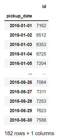
plt.figure(figsize=(8,5))
plt.plot(train.groupby('pickup_date').count()[['id']], 'o-',label='train')


plt.title("Distribution of Pickups over time")

There is a drop seen in the number of pick ups in end the January 2016
- 2016 년 1월 말에 택시를 타는 사람의 수가 감소
dropoff over the entire time period - 일별로 비교
어느 시기에 많이 하차했을까 ?
plt.figure(figsize=(8,5))
plt.plot(train.groupby('dropoff_date').count()[['id']], 'o-',label='train')


plt.title("Distribution of dropoff over time")
- 시간에 따른 승차하는 사람의 수와 비슷한 시기에 하락세를 보인다.
- 승차하는 사람의 수와 달리 하차하는 사람의 수는 2016년 7 월 달에 급격한 감소를 보인다.
→ 승차는 뉴욕에서 하지만 하차는 다른지역에서 한다 ?
What is the distribution of Trip distance
- 주행거리 (로그) 에 대한 분포
plt.figure(figsize=(8,5))
sns.kdeplot(np.log(train['trip_distance'].values)).set_title("Trip Distance Distribution")
plt.xlabel("Trip Distance (log)")
- Trip Distance (log) 가 0~1 인 경우가 많다.
Trip Duration vs Trip Distance
- 주행시간과 주행거리는 어떤 관계가 있을까 ?
plt.scatter(np.log(train['trip_distance'].values), np.log(train['trip_duration'].values),
              color='blue', label='train')
plt.title("Distribution of Trip Distance vs Trip Duration")
plt.xlabel("Trip Distance (log scale)")
plt.ylabel("Trip Duration (log scale)")
- 택시를 타고 이동한 거리가 길수록 택시 이용시간도 많아지는 경향이 있다.
Is the trip duration higher at different hours?
- 택시를 승차한 시각에 따른 택시 평균 이용시간
avg_duration_hour=train.groupby(['pickup_hour'])['trip_duration'].mean().reset_index().rename(columns={'trip_duration':'avg_trip_duration'})

avg_duration_hour  # 승차한 시각에 따른 택시 이용 시간 (초)
- '택시를 승차한 시각에 따른 평균 택시 이용시간' 그래프로 표현
plt.figure(figsize=(8,5))
plt.plot(train.groupby(['pickup_hour'])['trip_duration'].mean(),'o-')
Trip duration increases between 10 to 15 hours.
- 10시 15시에 택시를 타면 택시를 오래탄다.
- = 평균 'trip_duration' 기간이 길다.
Distribution of Pickups across Days
- 어느요일에 택시를 가장 많이 탈까 ?
plt.figure(figsize=(8,5))
sns.countplot(train['pickup_day_of_week'],order=['Monday','Tuesday','Wednesday','Thursday','Friday','Saturday', 'Sunday'])
The number of pickups are very low on Monday.
From Tuesday to Friday the number of pickups keep increasing
* 금요일까지 택시이용량이 점점 증가한다.
Avg Trip Duration over Days of week
- 요일별 평균 택시 이용시간 (초)
avg_duration_day=train.groupby(['pickup_day_of_week'])['trip_duration'].mean().reset_index().rename(columns={'trip_duration':'avg_trip_duration'})avg_duration_day
- '요일별 평균 택시 이용시간 (초)' 그래프로 표현
plt.figure(figsize=(8,5))
sns.barplot(x='pickup_day_of_week',y='avg_trip_duration',data=avg_duration_day,order=['Monday','Tuesday','Wednesday','Thursday','Friday','Saturday', 'Sunday']).set_title("Avg Trip Duration vs Pickup Days of Week")
- The highest average speed is on Thursday
* 목요일에 택시를 가장 오래 탄다.
Create a caluclated field Bearing - Bearing 변수 생성
Bearing measures the direction of travel
The formula is: θ = atan2( sin Δλ ⋅ cos φ2 , cos φ1 ⋅ sin φ2 − sin φ1 ⋅ cos φ2 ⋅ cos Δλ ) λ is the longitude
- 'Bearing' 변수 : 택시 주행 방향을 나타내는것 같음
- 택시가 어디 쪽으로 향하여 가는지 분석 ?
- 목적지에 관하여 예측 ?
def calculateBearing(lat1,lng1,lat2,lng2):
    R = 6371
    lng_delta_rad = np.radians(lng2 - lng1)
    lat1, lng1, lat2, lng2 = map(np.radians, (lat1, lng1, lat2, lng2))
    y = np.sin(lng_delta_rad) * np.cos(lat2)
    x = np.cos(lat1) * np.sin(lat2) - np.sin(lat1) * np.cos(lat2) * np.cos(lng_delta_rad)
    return np.degrees(np.arctan2(y, x))
위 공식에 따라 함수를 생성하고 train 데이터 셋에 'bearing' 이라는 변수 추가
train['bearing']=train.apply(lambda row:calculateBearing(row['pickup_latitude_round3'],row['pickup_longitude_round3'],row['dropoff_latitude_round3'],row['dropoff_longitude_round3']),axis=1)train['bearing'].head() # 'bearing' 변수 확인 0 98.823984
1 -119.053505
2 -159.948291
3 -173.347990
4 180.000000
Name: bearing, dtype: float64
Distribution of Bearing
- Bearing 변수의 분포를 알아보자.
sns.kdeplot(train['bearing'])
- -150 , 150의 값을 갖는 경우가 많다.
Bearing vs Trip Duration
- 방향 변수와 이용시간의 관계는 ?
plt.figure(figsize=(8,5))
plt.scatter(train['bearing'].values,y=np.log(train['trip_duration'].values))
plt.xlabel("Bearing")
plt.ylabel("Trip Duration (log scale)")
The outliers in trip duration are all around bearing -50 degrees
* bearing 변수가 대략 -50 의 값을 가질 때 택시 이용시간이 이상치를 갖는다.
- 'trip_duration' 변수의 이상치에 대하여 -
앞서 택시 이용시간 (초) 를 시간단위로 환산한 변수 'trip_duration_in_hour' 에서 이상치가 있음을 파악했었다.
→ 여행시간이 24 시간이 넘어가는 경우 4 개의 이상치가 있었다.

이를 참고하면
- bearing 변수가 -150 미만일 때 'trip_duration' 변수에 이상치가 1 개 존재하며
- bearing 변수가 대략 -50 의 값을 가질 때 'trip_duration' 변수에 이상치가 3 개 존재한다.
Distribution of Store and FWD Flag - 메모리 저장 여부
store_and_fwd_flag :
This flag indicates whether the trip record was held in vehicle memory before sending to the vendor,
aka “store and forward,” because the vehicle did not have a connection to the server.
* 주행 기록이 공급업체에 전송되기 전에 차량 메모리에 저장되었는지 여부를 나타냅니다.
* “store and forward,” : 링크로 전송하기 전에 저장을 한 뒤 전달 ; 저장 후 전달
- Y = store and forward
- N = not a store and forward trip
train['store_and_fwd_flag'].value_counts() N 1450599
Y 8045
Name: store_and_fwd_flag, dtype: int64
- 주행기록이 공급업체에 전송되기 전에 차량 메모리가 저장이 되지 않은 경우가 더 많다.
train.loc[train['store_and_fwd_flag']=='Y','trip_duration'] # 'store_and_fwd_flag'] 가 'Y' 일 때의 택시이용시간 (초) 348 918
491 629
610 926
774 892
846 717
...
1457556 1279
1457670 2228
1457897 1170
1458060 2156
1458416 592
Name: trip_duration, Length: 8045, dtype: int64
- 메모리 저장 여부에 따른 이용시간 (log) 분포
plt.figure(figsize=(8,5))
sns.kdeplot(np.log(train.loc[train['store_and_fwd_flag']=='Y','trip_duration'].values),label= 'Store and Fwd =Yes')
sns.kdeplot(np.log(train.loc[train['store_and_fwd_flag']=='N','trip_duration'].values),label= 'Store and Fwd =No')

plt.title("Distribution of  Store and Fwd Flag vs Trip Duration(log scale)")
plt.xlabel('Trip Duration (log scale)')
plt.ylabel('Density')
- 두 경우 모두 이용시간이 4~8 일 때 높게 나타난다. 두 분포는 비슷한 경향을 보인다.
- record 를 저장하지 않은 경우가 더 높다. ( log Trip Duration 이 4 ~ 7 일 때 )
Group Locations into cluster
This will help creating neighbourhoods.
And pickups from certain neightbourhoods may have a longer trip duration
* 특정 지역에서 택시를 타는 사람이 택시를 더 오래 이용할수도 있다.
Kmeans 클러스터링
- https://velog.io/@jhlee508/%EB%A8%B8%EC%8B%A0%EB%9F%AC%EB%8B%9D-K-%ED%8F%89%EA%B7%A0K-Means-%EC%95%8C%EA%B3%A0%EB%A6%AC%EC%A6%98
- 비슷한 특성을 지닌 데이터들끼리 묶어 K개의 군집으로 군집화하는 대표적인 군집화 기법
- KMeans 클러스터링을 적용하여 택시타는 곳에 대한 군집을 만들어보자.
coords = np.vstack((train[['pickup_latitude', 'pickup_longitude']].values,
                    train[['dropoff_latitude', 'dropoff_longitude']].values,
                    test[['pickup_latitude', 'pickup_longitude']].values,
                    test[['dropoff_latitude', 'dropoff_longitude']].values))
kmeans = KMeans(n_clusters=8, random_state=0).fit(coords)

train.loc[:, 'pickup_neighbourhood'] = kmeans.predict(train[['pickup_latitude', 'pickup_longitude']])
train.loc[:, 'dropoff_neighbourhood'] = kmeans.predict(train[['dropoff_latitude', 'dropoff_longitude']])

city_long_border = (-74.03, -73.75)
city_lat_border = (40.63, 40.85)
fig, ax = plt.subplots(ncols=1, sharex=True, sharey=True)
ax.scatter(train['pickup_longitude'], train['pickup_latitude'],
              c=train['pickup_neighbourhood'], label='train', alpha=0.1)

fig.suptitle('Pickup Neighbourhood')

ax.set_ylabel('latitude')
ax.set_xlabel('longitude')
plt.ylim(city_lat_border)
plt.xlim(city_long_border)
train['pickup_neighbourhood'] 0 0
1 0
2 0
3 3
4 6
..
1458639 0
1458640 0
1458641 6
1458642 0
1458643 6
Name: pickup_neighbourhood, Length: 1458644, dtype: int32
- 각 데이터들이 어떤 군집에 들어갔는지 확인
Number of pickups in each neighbourhood
- 어떤 군집에 가장 수가 많을까 ?
plt.figure(figsize=(8,5))
sns.countplot(train['pickup_neighbourhood']).set_title("Distribution of Number of Pickups across Neighbourhoods")
- 0 집단에 데이터가 가장 많이 분포한다. → 0 집단의 특성을 지닌 데이터가 많음
- 0 집단 다음으로 4, 5 집단에 데이터가 많이 분포한다.
- 분류된 군집에 따른 택시 이용시간은 어떠할까 ?
avg_duration_neighbourhood=train.groupby(['pickup_neighbourhood'])['trip_duration'].mean().reset_index().rename(columns={'trip_duration':'avg_trip_duration'})
plt.figure(figsize=(8,5))
sns.barplot(x='pickup_neighbourhood',y='avg_trip_duration',data=avg_duration_neighbourhood).set_title("Avg Trip Duration vs Neighbourhood")
Neighbourhood 2 has very high average Trip duration, though Neighbourhood 0 has majority of pickups
* 0 집단의 수가 가장 많았음에도 불구하고 2집단의 택시 이용시간이 가장 길다.
Building Models
From the training data we need to drop "dropoff datetime features".
We also only keep lat lng rounded to 3 decimal places
- train / test 데이터의 일부 변수 제거 후 training / testing 데이터 생성
제거하는 변수
- 'avg_speed_kph'
- 'trip_duration_in_hour'
- 'dropoff_date'
- 'dropoff_day'
- 'dropoff_hour'
- 'dropoff_day_of_week'
- 'dropoff_datetime'
- 'pickup_latitude'
- 'pickup_longitude'
- 'dropoff_latitude'
- 'dropoff_longitude'
drop_cols=['avg_speed_kph','trip_duration_in_hour','dropoff_date','dropoff_day','dropoff_hour','dropoff_day_of_week','dropoff_datetime','pickup_latitude','pickup_longitude','dropoff_latitude','dropoff_longitude']
training=train.drop(drop_cols,axis=1)
testing=test.drop(['pickup_latitude','pickup_longitude','dropoff_latitude','dropoff_longitude'],axis=1)
- 'trip_duration' 에 로그를 취한 'log_trip_duration' 변수 생성
We have to predict trip_duration. We will convert this to log scale and predict
training['log_trip_duration']=training['trip_duration'].apply(lambda x:np.log(x))
training.drop(['trip_duration'],axis=1,inplace=True)
print("Training Data Shape ",training.shape)
print("Testing Data Shape ",testing.shape) Training Data Shape (1458644, 18)
Testing Data Shape (625134, 17)
- 요일변수 수치화
Let us also encode day of week as numbers
def encodeDays(day_of_week):
    day_dict={'Sunday':0,'Monday':1,'Tuesday':2,'Wednesday':3,'Thursday':4,'Friday':5,'Saturday':6}
    return day_dict[day_of_week]
training['pickup_day_of_week']=training['pickup_day_of_week'].apply(lambda x:encodeDays(x))
testing['pickup_day_of_week']=testing['pickup_day_of_week'].apply(lambda x:encodeDays(x))
- trainig , testing 데이터 저장
training.to_csv("C://Input/input_training.csv",index=False)
testing.to_csv("C://Input/input_testing.csv",index=False)
del training
del testing
del train
del test
- 범주형 변수 수치화 하기 ( 범주가 2개 이하인 경우만 )
def LabelEncoding(train_df,test_df,max_levels=2):
    for col in train_df:
        if train_df[col].dtype == 'object':
            if len(list(train_df[col].unique())) <= max_levels:
                le = preprocessing.LabelEncoder()  # 범주형 데이터 변환
                le.fit(train_df[col])
                train_df[col]=le.transform(train_df[col])
                test_df[col]=le.transform(test_df[col])
    return [train_df,test_df]
- 데이터 타입이 'object' 인 경우 -
training.info()training['id'].unique()training['pickup_date'].unique()training['store_and_fwd_flag'].unique()- 수치화 코드 이해 -
if training['store_and_fwd_flag'].dtype == 'object':
            if len(list(training['store_and_fwd_flag'].unique())) <= 2:
                le = preprocessing.LabelEncoder()   # 문자를 숫자형으로 변경
                le.fit(training['store_and_fwd_flag'])
                training['store_and_fwd_flag2']=le.transform(training['store_and_fwd_flag'])
testing['store_and_fwd_flag2']=le.transform(testing['store_and_fwd_flag'])training['store_and_fwd_flag2'].unique()- 각 데이터셋 (train/test) 에는 없는 변수값을 0 으로 바꾸기
def readInputAndEncode(input_path,train_file,test_file,target_column):
    training=pd.read_csv(input_path+train_file)
    testing=pd.read_csv(input_path+test_file)

    training,testing=LabelEncoding(training,testing)   # 위에서 만들었던 함수 적용

    #print("Training Data Shape after Encoding ",training.shape)
    #print("Testing Data Shape after Encoding ",testing.shape)
    #Check if all train columns are there in test data. If not add the column to test data and replace it with zero
    train_cols=training.columns.tolist()   # 각 컬럼을 리스트로
    test_cols=testing.columns.tolist()
    col_in_train_not_test=set(train_cols)-set(test_cols)   # test 데이터에는 없는 변수 추출

    for col in col_in_train_not_test:
        if col!=target_column:
            testing[col]=0     # 택시 이용시간 변수가 아니면 test 데이터의 그 변수값은 0 으로 지정

    col_in_test_not_train=set(test_cols)-set(train_cols)  # train 데이터에는 없는 변수
    for col in col_in_test_not_train:
        training[col]=0        # train 데이터에는 없는 변수값은 모두 0 으로 지정

    print("Training Data Shape after Processing ",training.shape)
    print("Testing Data Shape after Processing ",testing.shape)
    return [training,testing]
train,test=readInputAndEncode("C://Input/",'input_training.csv','input_testing.csv','log_trip_duration')
train.drop(['pickup_date'],axis=1,inplace=True)
test.drop(['pickup_date'],axis=1,inplace=True)
train.drop(['pickup_datetime'],axis=1,inplace=True)
test.drop(['pickup_datetime'],axis=1,inplace=True)
test_id=test['id']
train.drop(['id'],axis=1,inplace=True)
test.drop(['id'],axis=1,inplace=True)
Training Data Shape after Processing (1458644, 18)
Testing Data Shape after Processing (625134, 17)
- train 과 'log_trip_duration' (타겟변수) 를 훈련 / 검증 데이터셋으로 나누기
def GetFeaturesAndSplit(train,test,target,imputing_strategy='median',split=0.25,imputation=True):   # 결측치 평균으로 대체
    labels=np.array(train[target])   # 'log_trip_duration' 변수의 값 = labels
    training=train.drop(target, axis = 1)
    training = np.array(training)
    testing=np.array(test)
    if imputation==True:
        imputer=Imputer(strategy=imputing_strategy,missing_values=np.nan)  #  missing_values에 대치하고자 하는 값을 지정
        imputer.fit(training)
        training=imputer.transform(training)
        testing=imputer.transform(testing)
    train_features, validation_features, train_labels, validation_labels = train_test_split(training, labels, test_size = split, random_state = 42)
    return [train_features,validation_features,train_labels,validation_labels,testing]
train_features,validation_features,train_labels,validation_labels,testing=GetFeaturesAndSplit(train,test,'log_trip_duration',imputation=False)
'파이썬 > 캐글 필사' 카테고리의 다른 글
| Tackling Toxic Using Keras 데이터 (0) | 2022.02.17 |
|---|---|
| Porto Seguro’s Safe Driver Prediction 데이터 (0) | 2022.02.05 |
| Titanic 데이터 (0) | 2022.01.26 |


