이번 포스팅에서는 빈도 / 비교 분석에 대하여 다룰 예정입니다.
이후 포스팅에서 감정분석도 진행하니 참고해주세요.
빈도분석 , 비교분석
- Spider , Matrix , Snowden 범주 별 최다 빈도 수 단어 분석
- 로그 오즈비로 Spider , Matrix 두 집단 비교
- tf-idf로 세 집단 비교
Movie Review And Rating
https://www.kaggle.com/newra008/movie-review-and-rating
Movie Review And Rating
Movies review from year 2016-2022
www.kaggle.com

ID : Id provided for each movie review
Movie : Name of the movie
Year : The release year of the movie
Genres : Genres of the movie i.e. Action, sci-fi, horror, etc
Review : Raw review consisting of text and emoji
Rating : Rating varies from 1 to 5
필요한 라이브러리
library(readr)
library(dplyr)
library(stringr)
library(tidytext)
library(ggplot2)
데이터 불러오기
# 영화리뷰 데이터 불러오기
Movie_review <- read_csv("C://WORK/R/Movie Review And Rating.csv")
head(Movie_review)

영화 제목에 따라 데이터 분류
영화 별로 단어 빈도를 비교해야 하므로 영화 제목에 따라 데이터를 분류하여 새로운 데이터셋을 생성한다.
여기서 변수를 3개로 지정했는데 ( 로그오즈비 사용, TF_IDF 사용을 위해 3개 정도로 지정했다. )
"Spider-Man: No Way Home" , "The Matrix Resurrections" , "Snowden" 을 대상으로 분석을 시행하였다.
- Spider 데이터
Spider_review<-Movie_review %>% filter(Movie=="Spider-Man: No Way Home")
Spider <-Spider_review$Review

- filter 함수에 영화 이름이 "Spider-Man: No Way Home" 일 때의 조건을 주었음
- 다음과 같이 스파이더 맨 영화에 대한 데이터만 추출됐음을 확인할 수 있다.
- Matrix 데이터
Matrix_review<-Movie_review %>% filter(Movie=="The Matrix Resurrections")
Matrix<-Matrix_review$Review
head(Matrix_review)

- Snowden 데이터
Snowden_review<-Movie_review %>% filter(Movie=="Snowden")
Snowden<-Snowden_review$Review
head(Snowden_review)

이후 사용되는 영어 형태소 분석 패키지 : stopwords("en") 에서는 소문자만 인식하기 때문에 소문자로 변경한다.
- tolower : 소문자로 변경
- toupper : 대문자로 변경
# 데이터 소문자로 전환
Spider<-tolower(Spider)
Matrix<-tolower(Matrix)
Other<-tolower(Snowden)
소문자로 바뀐 Other 데이터

데이터 전처리
- 영어 외의 문자들을 공백으로 처리하고 , 이로 인해 생기는 중복공백을 제거
# 불필요한 문자 제거하기

# Spider 데이터
Spider <- Spider %>%
str_replace_all("[^A-z]"," ") %>%  # A-z 를 제외한 문자들을 공백으로 대체
str_squish() %>%   # 연속된 공백 제거
as_tibble()
head(Spider)

# Matrix 데이터
Matrix <- Matrix %>%
str_replace_all("[^A-z]"," ") %>%  # A-z 를 제외한 문자들을 공백으로 대체
str_squish() %>%   # 연속된 공백 제거
as_tibble()
head(Matrix)

# Snowden 데이터
Snowden <- Snowden %>%
str_replace_all("[^A-z]"," ") %>%  # A-z 를 제외한 문자들을 공백으로 대체
str_squish() %>%   # 연속된 공백 제거
as_tibble()
head(Snowden)

- 여기서 I'm , He's 등 ' (apostrophe) 도 같이 제외된다.
토큰화 하기
- 띄어쓰기 기준 토큰화
# 토큰화 하기
token_Spider <- Spider %>%
unnest_tokens(input = value, output = word, token = "words")  # 띄어쓰기 기준 토큰화


token_Matrix <- Matrix %>%
unnest_tokens(input = value, output = word, token = "words")  # 띄어쓰기 기준 토큰화


token_Snowden <- Snowden %>%
unnest_tokens(input = value, output = word, token = "words")  # 띄어쓰기 기준 토큰화


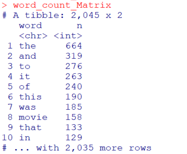
- 데이터 전처리를 했으나 분석에 의미없는 단어들 ( ex : is , by, or, it ... ) 이 존재한다.
단어빈도 구하기
# 단어빈도 구하기
word_count_Spider <-token_Spider %>%
count(word,sort=T) # 내림차순 정렬
word_count_Spider


word_count_Spider <-word_count_Spider %>%
filter(str_count(word)>1)  # 한 글자로 된 단어 제거
word_count_Spider


word_count_Matrix <-token_Matrix %>%
count(word,sort=T) # 내림차순 정렬
word_count_Matrix


word_count_Matrix <-word_count_Matrix %>%
filter(str_count(word)>1)  # 한 글자로 된 단어 제거
word_count_Matrix


word_count_Snowden <-token_Snowden %>%
count(word,sort=T) # 내림차순 정렬
word_count_Snowden


word_count_Snowden <-word_count_Snowden %>%
filter(str_count(word)>1)  # 한 글자로 된 단어 제거
word_count_Snowden
단어의 빈도가 높은 순대로 나오도록 내림차순 정렬 후
한 글자로 된 단어는 제거하였다. (분석에 의미없는 단어가 대부분이기 때문)
- Spider 데이터


- Matirx 데이터

- Snowden 데이터


빈도수가 높은 상위 20 개의 단어 추출
# 단어 사용 빈도가 높은 20개 추출
top20_Spider <- word_count_Spider %>% head(20)
top20_Spider

top20_Matrix <- word_count_Matrix %>% head(20)
top20_Matrix

top20_Snowden <- word_count_Snowden %>% head(20)
top20_Snowden


막대 그래프를 통한 상위 빈도 단어 시각화
# 단어 사용 빈도가 높은 단어 20개의 막대그래프
ggplot(top20_Spider, aes(x = reorder(word, n), y = n)) +
 geom_col() +
 coord_flip() +
 geom_text(aes(label = n), hjust = -0.3) +            # 막대 밖 빈도 표시

 labs(title = "Spider 영화 리뷰 단어 빈도",  # 그래프 제목
      x = NULL, y = NULL) +                           # 축 이름 삭제

 theme(title = element_text(size = 12))               # 제목 크기


ggplot(top20_Matrix, aes(x = reorder(word, n), y = n)) +
 geom_col() +
 coord_flip() +
 geom_text(aes(label = n), hjust = -0.3) +            # 막대 밖 빈도 표시

 labs(title = "Matrix 영화 리뷰 단어 빈도",  # 그래프 제목
      x = NULL, y = NULL) +                           # 축 이름 삭제

 theme(title = element_text(size = 12))               # 제목 크기


ggplot(top20_Snowden, aes(x = reorder(word, n), y = n)) +
 geom_col() +
 coord_flip() +
 geom_text(aes(label = n), hjust = -0.3) +            # 막대 밖 빈도 표시

 labs(title = "Snowden 영화 리뷰 단어 빈도",  # 그래프 제목
      x = NULL, y = NULL) +                           # 축 이름 삭제

 theme(title = element_text(size = 12))               # 제목 크기
- Spider 데이터

- Matirx 데이터

- Snowden 데이터
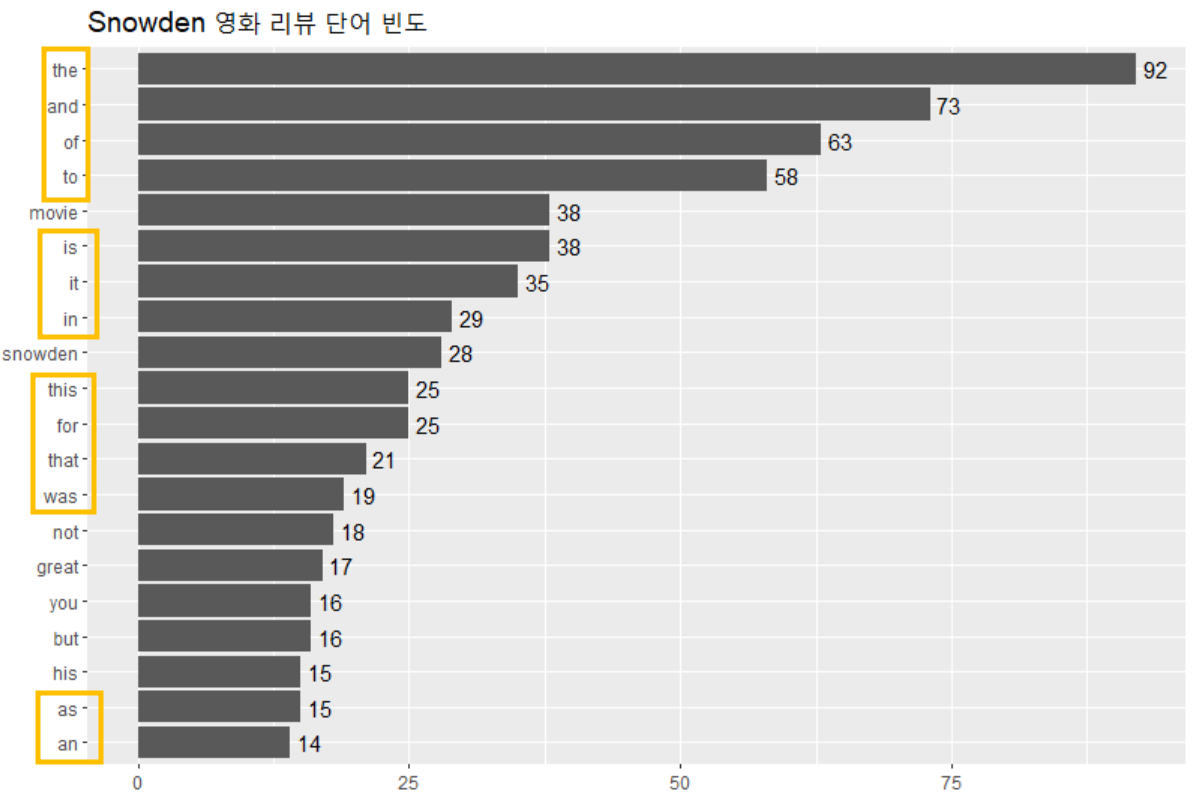
- 대부분의 단어들이 관사, 전치사 등으로 유의미하다고 볼 수 없다.
- 따라서 다른 방법의 전처리가 필요하다.
영어 형태소 분석을 위한 패키지 설치
이전의 빈도 분석에서 사용했던 KoNLP 패키지는 한국어 형태소 패키지로 영어 분석에서는 사용할 수 없다.
영어 형태소 분석 시에는 tm ( Text Mining ) 패키지를 많이 사용한다.
install.packages("tm")
library(tm)
유의미하지 않은 관사, 전치사, 접속사, 조사 등 불용어 (tm 패키지)
stopwords("en")

전처리를 위한 tm 패키지 함수
- removeWords : 단어를 제거해준다.
- removeWords(text, stopwords("en")) : text 에서 stopwords("en") 를 참고하여 불용어 제거
- removePunctuation(text) : 구두점을 제거해준다. ( ' ; apostrophe 도 제거한다. )
문장 i'm student. !? 을 예시로 보면
removeWords(text, stopwords("en")) 으로 불용어 i'm 을 먼저 제거해주는 것이 효율적이다.
→ removePunctuation(text) 가 ' ; apostrophe 도 제거하기 때문 이다.
어근 추출
job - ,jobs 또는 like - liked - likely 와 같이 단수/ 복수나 시제가 다른 단어는 같은 단어로 인식하는 것이 효과적이다.
이러한 문제는 어근만 추출하여 원형으로 전환시켜 주어 해결한다.
Snowball 패키지 설치
영어 형태소 분석시 사용된다.
install.packages("SnowballC")
library(SnowballC)
Snowball 패키지 함수
- stemDocument : 어근만 추출하여 시제, 복수형 등을 제거해준다.
- stemCompletion : dictionary 를 통해 불완전한 단어를 완전하게 바꿔준다.
- stemCompletion
stemCompletion(x,        # 바꿔줄 문자 벡터
               dictionary      # 참고할 문자 벡터
               type = c("Prevalent",   # dictionary 중 빈도가 가장 높은 단어 (기본값)
                        "first",     # dictionary 중 첫 번째 단어
                        "longest"   # dictionary 중 가장 긴 단어
                        "none"     # 변경하지 않음
                        "random"    # dictionary 중 랜덤
                        "shortest"))   # dictionary 중 가장 짧은 단어
test<-stemDocument(c("updated","update","updating"))
test
[1] "updat" "updat" "updat"
stemCompletion(test,dictionary=c("updated","update","updating")) updat updat updat
"update" "update" "update"
데이터 전처리
- 전처리 전의 Spider 데이터

- 전처리 전의 Matirx 데이터

- 전처리 전의 Snowden 데이터

- 한 글자의 단어 , 특수문자 (이모티콘) , 관사 등이 나타나 전처리가 필요해 보인다.
- 'tm' 패키지와 'SnowballC' 패키지를 이용하여 전처리를 진행하기로 하였다.
1. Dictionary 만들기
# Dictionary 만들기
dict_Spider <- Spider %>%
removeWords(stopwords("en")) %>%   # 불용어 제거
removePunctuation()  %>%               # 구두점 제거
removeNumbers() %>%                   # 숫자 제거
str_squish() %>%
as_tibble() %>%
unnest_tokens(input = value, output = word, token="words")  %>%
anti_join(stop_words)  %>%    # 불용어를 먼저 제거하고 어근을 추출
unlist() %>%
as.character ()  # stemCompletion 에서는 데이터를 character vector 형태로 사용


dict_Matrix <- Matrix %>%
removeWords(stopwords("en")) %>%   # 불용어 제거
removePunctuation()  %>%               # 구두점 제거
removeNumbers() %>%                   # 숫자 제거
str_squish() %>%
as_tibble() %>%
unnest_tokens(input = value, output = word, token="words")  %>%
anti_join(stop_words)  %>%    # 불용어를 먼저 제거하고 어근을 추출
unlist() %>%
as.character ()  # stemCompletion 에서는 데이터를 character vector 형태로 사용


dict_Other <- Snowden %>%
removeWords(stopwords("en")) %>%   # 불용어 제거
removePunctuation()  %>%               # 구두점 제거
removeNumbers() %>%                   # 숫자 제거
str_squish() %>%
as_tibble() %>%
unnest_tokens(input = value, output = word, token="words")  %>%
anti_join(stop_words)  %>%    # 불용어를 먼저 제거하고 어근을 추출
unlist() %>%
as.character ()  # stemCompletion 에서는 데이터를 character vector 형태로 사용
Joining , by = "word"
- StemCompletion 에 이용하기 위해 Dictionary 를 만든다.
2. 불용어 , 구두점, 숫자 제거
Spider <- Spider %>%
removeWords(stopwords("en")) %>%   # 불용어 제거
removePunctuation()  %>%               # 구두점 제거
removeNumbers() %>%                   # 숫자 제거
str_squish() %>%
as_tibble()

Spider


Matrix <- Matrix %>%
removeWords(stopwords("en")) %>%   # 불용어 제거
removePunctuation()  %>%               # 구두점 제거
removeNumbers() %>%                   # 숫자 제거
str_squish() %>%
as_tibble()

Matrix


Snowden <- Snowden %>%
removeWords(stopwords("en")) %>%   # 불용어 제거
removePunctuation()  %>%               # 구두점 제거
removeNumbers() %>%                   # 숫자 제거
str_squish() %>%
as_tibble()

Snowden
- 제거 전 Spider

- 제거 후 Spider

- 제거 전 Matrix

- 제거 후 Matrix

- 제거 전 Snowden

- 제거 후 Snowden

- 분석시 의미없는 문자들이 제거됐음을 확인할 수 있다.
3. 토큰화
token_Spider <- Spider %>%
unnest_tokens(input = value, output = word, token="words")  %>%
anti_join(stop_words)  %>%    # 불용어를 먼저 제거하고 어근을 추출
unlist() %>%
as.character () %>%  # stemCompletion 에서는 데이터를 character vector 형태로 사용
stemDocument()   # 어근 추출

token_Spider


token_Matrix <- Matrix %>%
unnest_tokens(input = value, output = word, token="words")  %>%
anti_join(stop_words)  %>%    # 불용어를 먼저 제거하고 어근을 추출
unlist() %>%
as.character () %>%  # stemCompletion 에서는 데이터를 character vector 형태로 사용
stemDocument()   # 어근 추출

token_Matrix


token_Snowden <- Snowden %>%
unnest_tokens(input = value, output = word, token="words")  %>%
anti_join(stop_words)  %>%    # 불용어를 먼저 제거하고 어근을 추출
unlist() %>%
as.character () %>%  # stemCompletion 에서는 데이터를 character vector 형태로 사용
stemDocument()   # 어근 추출

token_Snowden

- stemDocument 함수를 이용하여 어근을 추출한다.
- anti_joint(stop_words) 으로 불용어를 먼저 제거해준 다음 어근을 추출한다.
- stemCompletion 함수에서는 데이터를 character vector 형태로 사용한다.
+ 어근을 먼저 추출하고 불용어 제거시 단어의 형태가 어근이 형태로 모두 제거되지 않는다.
4. stemCompletion 함수를 이용하여 완전한 단어로 변환
# stemCompletion 함수를 이용하여 완전한 단어로 변환
word_noun_Spider <- stemCompletion(token_Spider, dictionary=dict_Spider) %>%
as_tibble()

word_noun_Spider


word_noun_Matrix <- stemCompletion(token_Matrix, dictionary=dict_Matrix) %>%
as_tibble()

word_noun_Matrix


word_noun_Snowden <- stemCompletion(token_Snowden, dictionary=dict_Snowden) %>%
as_tibble()

word_noun_Snowden
Spider 데이터

Matirx 데이터

Snowden 데이터

+ stemCompletion 함수를 이용하여 전처리를 하여도 한계가 존재한다.

다음과 같이 완전한 단어로 변환시킨 결과값이 "" 으로 존재하는 단어들이 있다
> head(token_Matrix,10)
[1] "pretti" "entertainingsur" "dialog" "viewer" "ve"
[6] "confus" "movi" "pretti" "bad" "review"
Matrix 데이터에 토큰화 후 어근추출 결과, "pretii" 라는 단어가 이 경우에 해당되었다.
이는 사전에 정의한 dictionary 를 통해 단어를 바꿔주지 못하였음을 뜻하는것 같다.
단어 빈도수 구하기
# 단어 빈도수 구하기
word_count_Spider <- word_noun_Spider  %>%
count(value, sort =T)  %>%   # 내림차순
filter(str_count(value)>1)  # 두 글자 이상


word_count_Matrix <- word_noun_Matrix  %>%
count(value, sort =T)  %>%   # 내림차순
filter(str_count(value)>1)  # 두 글자 이상


word_count_Snowden <- word_noun_Snowden  %>%
count(value, sort =T)  %>%   # 내림차순
filter(str_count(value)>1)  # 두 글자 이상


빈도수가 높은 상위 20개의 단어 추출
# 단어 빈도 수 높은 20개 단어 구하기
top20_Spider <-word_count_Spider %>% head(20)

top20_Matrix <-word_count_Matrix %>% head(20)

top20_Other <-word_count_Other %>% head(20)


빈도가 높은 상위 20 개의 단어 막대그래프 시각화
# 단어 사용 빈도가 높은 단어 20개의 막대그래프
ggplot(top20_Spider, aes(x = reorder(value, n), y = n)) +
 geom_col() +
 coord_flip() +
 geom_text(aes(label = n), hjust = -0.3) +            # 막대 밖 빈도 표시

 labs(title = "Spider 영화 리뷰 단어 빈도",  # 그래프 제목
      x = NULL, y = NULL) +                           # 축 이름 삭제

 theme(title = element_text(size = 12))               # 제목 크기


ggplot(top20_Matrix, aes(x = reorder(value, n), y = n)) +
 geom_col() +
 coord_flip() +
 geom_text(aes(label = n), hjust = -0.3) +            # 막대 밖 빈도 표시

 labs(title = "Matrix 영화 리뷰 단어 빈도",  # 그래프 제목
      x = NULL, y = NULL) +                           # 축 이름 삭제

 theme(title = element_text(size = 12))               # 제목 크기


ggplot(top20_Snowden, aes(x = reorder(value, n), y = n)) +
 geom_col() +
 coord_flip() +
 geom_text(aes(label = n), hjust = -0.3) +            # 막대 밖 빈도 표시

 labs(title = "Snowden 영화 리뷰 단어 빈도",  # 그래프 제목
      x = NULL, y = NULL) +                           # 축 이름 삭제

 theme(title = element_text(size = 12))               # 제목 크기


로그 오즈비를 이용한 비교 분석
두 영화 Spider 와 Matrix 에서 상대적으로 많이 나온 단어를 비교해 보려고 한다.
dplyr 패키지의 mutate() 함수 알아보기
: 데이터 프레임 자료형에 새로운 파생 column을 만드는 함수
데이터에 movie 변수 추가
#영화 리뷰 데이터
library(dplyr)


word_count_Spider <- word_count_Spider %>%   # 영화 Spider
        mutate(movie = "spider")   # 영화 이름 변수 추가

word_count_Matrix <- word_count_Matrix %>%   # 영화 Spider
        mutate(movie = "matrix")   # 영화 이름 변수 추가


두 데이터 합치기
bind_row() 를 이용해 두 데이터를 행(세로) 방향으로 결합
# Spider , Matrix 리뷰 데이터 합치기
movie <- bind_rows(word_count_Spider,word_count_Matrix)   # 두 데이터를 행 방향으로 결합

long form 을 wide form 으로 변형하기
tidyr 패키지의 pivot_wider () 을 이용해 long form 데이터를 가로로 넓은 형태의 wide form 데이터로 변형하겠다.
wide form
- 단어가 두 연설문에 몇 번씩 사용되었는지 비교하기 쉽다.
- 변수를 이용해 연산하기 수월하다.
pivot_wider()에는 다음과 같은 파라미터를 입력한다
- names_form : 변수명으로 만들 값이 들어있는 변수.
여기서는 president 에 들어있는 "lee","roh" 을 변수명으로 만들어야 하므로 president 를 입력
- values_form : 변수에 채워 넣을 값이 들어 있는 변수. 여기서는 변수에 단어 빈도를 채워 넣어야 하므로 n을 입력
출력 결과를 보면, 한 단어가 한 행으로 구성되므로 단어가 두 영화 리뷰에 몇 번 사용되었는지 쉽게 비교할 수 있다.
NA를 0 으로 바꾸기
NA 이면 연산할 수 없으므로 0 으로 변환해야 한다.
pivot_wider() 의 values_fill 에 list(n=0) 을 입력하면 Na = 0 으로 변환한다.
# 리뷰 단어 빈도를 wide form 으로 변환하기
library(tidyr)
movie_wide<- movie %>%
  pivot_wider(names_from = movie,
              values_from = n,
              values_fill = list(n = 0))  # NA=0 으로 반환한다.

movie_wide

로그 오즈비 변수 추가
# 로그 오즈비 변수 추가
movie_wide <- movie_wide %>%
  mutate(log_odds_ratio = log(((spider + 1) / (sum(spider + 1))) /
                              ((matrix + 1) / (sum(matrix + 1)))))
로그 오즈비를 이용해 중요한 단어 비교하기
우선 group_by() 와 ifelse() 를 이용해 log_odds_ratio 가 0보다 크면 "Spider" 그렇지 않으면 "Matrix" 을 부여한다.
movie변수를 만들어 항목별로 분리한다.
그런 다음 slice_max() 와 abs() 를 이용해 log_odds_ratio의 절대값 기준으로 상위 10개 단어를 추출한다.
이렇게 하면 log_odds_ratio 가 "Spider" 에서 가장 큰 단어 10개, "Matirx" 에서 가장 작은 단어 10개를 추출한다.
# 로그 오즈비를 이용해 중요한 단어 비교하기
top10 <- movie_wide %>%
  group_by(movie = ifelse(log_odds_ratio > 0, "Spider", "Matrix")) %>%
  slice_max(abs(log_odds_ratio), n = 10, with_ties = FALSE)  # 상위 10개 단어 추출

top10 %>%
  arrange(-log_odds_ratio) %>%
  select(value, log_odds_ratio, movie)
로그 오즈비의 막대그래프
# 막대 그래프 만들기
library(ggplot2)
ggplot(top10, aes(x = reorder(value, log_odds_ratio),
                  y = log_odds_ratio,
                  fill = movie)) +
  geom_col() +
  coord_flip() +
  labs(x = NULL) +
  theme(text = element_text(family = "nanumgothic"))
TF _IDF 를 이용한 비교 분석
TF_IDF 를 이용하여 Spider , Matirx , Snowden 의 영화에서
각각 상대적으로 어떤 단어가 빈도가 높은지 알아보자.
1. 세 개의 데이터셋 합치기
word_count_Spider <- word_count_Spider %>%   # 영화 Spider
        mutate(movie = "spider")   # 영화 이름 변수 추가

word_count_Matrix <- word_count_Matrix %>%   # 영화 Matrix
        mutate(movie = "matrix")   # 영화 이름 변수 추가

word_count_Snowden <- word_count_Snowden %>%   # 영화 Snowden
        mutate(movie = "snowden")   # 영화 이름 변수 추가

# Spider , Matrix , Snowden 리뷰 데이터 합치기
movie <- bind_rows(word_count_Spider,word_count_Matrix,word_count_Snowden)
2. TF-IDF 구하기
tidytext 패키지의 bind_tf_idf() 를 이용하면 TF_IDF 를 구할 수 있다.
bind_tf_idf () 의 파라미터
- term : 단어
- document : 텍스트 구분 기준
- n : 단어 빈도
movie 를 bind_tf_idf() 에 적용해 TF-IDF 를 구한 다음, tf_idf 가 높은 순으로 정렬
# TF-IDF
movie<- movie %>%
  bind_tf_idf(term = value,           # 단어
              document = movie,  # 텍스트 구분 변수
              n = n) %>%             # 단어 빈도
  arrange(-tf_idf)   # 내림차순 정렬

TF - IDF 가 높은 단어 살펴보기
TF_IDF 를 이용하면 텍스트의 특징을 드러내는 중요한 단어가 무엇인지 파악할 수 있다.
tf_idf 가 높은 단어를 살펴보면 각 영화 리뷰가 다른 리뷰와 달리 무엇을 강조했는지 알 수 있다.
# TF-IDF 가 높은 단어 살펴보기
movie %>% filter(movie== "spider")
movie %>% filter(movie== "matrix")
movie %>% filter(movie== "snowden")
- Spider 데이터

- Matrix 데이터

- Snowden 데이터

3. 막대 그래프 만들기
각 영화 리뷰에서 TF-IDF 가 높은 단어를 추출하여 막대그래프로 시각화
- 상위 10개 단어 추출
top10 <- movie %>%
  group_by(movie) %>%
  slice_max(tf_idf, n = 10, with_ties = FALSE)   # 상위 10개의 단어 추출
- 막대그래프
# 막대 그래프 만들기
ggplot(top10, aes(x = reorder_within(value, tf_idf, movie),  # 그래프별로 축 정렬
                  y = tf_idf,
                  fill = movie)) +
  geom_col(show.legend = F) +
  coord_flip() +
  facet_wrap(~ movie, scales = "free", ncol = 3) +  # x축과 y축의 크기를 그래프 별로 정함
  scale_x_reordered() +   # 변수 항목 이름 제거
  labs(x = NULL) +  # x 축 이름 삭제
  theme(text = element_text(family = "nanumgothic")) # 폰트
+ 코드 총정리
'R > 텍스트 마이닝' 카테고리의 다른 글
| 영문 데이터에 대한 텍스트 마이닝 - 2 with 캐글 영화 리뷰 데이터 (0) | 2022.02.28 |
|---|---|
| KoNLP 패키지 설치 문제 해결 (0) | 2022.02.14 |
| 04. 감정분석 - 실습 (0) | 2022.02.14 |
| 04. 감정분석 (0) | 2022.02.14 |
| 03. 비교분석 - 실습 (0) | 2022.02.07 |


