Python Machine Learning (2019, 3rd ed., Sebastian Raschka, Vahid Mirjalili)
Chapter 1 Giving Computers the Ability to Learn from Data
Overview
- 1.1 Building intelligent machines to transform data into knowledge
- 1.2 The three different types of machine learning
- 1.2.1 Making predictions about the future with supervised learning
- Classification for predicting class labels
- Regression for predicting continuous outcomes
- 1.2.2 Solving interactive problems with reinforcement learning
- 1.2.3 Discovering hidden structures with unsupervised learning
- Finding subgroups with clustering
- Dimensionality reduction for data compression
- 1.2.1 Making predictions about the future with supervised learning
- 1.3 Introduction to the basic terminology and notations
- 1.4 A roadmap for building machine learning systems
- 1.4.1 Preprocessing - getting data into shape
- 1.4.2 Training and selecting a predictive model
- 1.4.3 Evaluating models and predicting unseen data instances
- 1.5 Using Python for machine learning
- 1.6 Summary
1.1 Building intelligent machines to transform data into knowledge
In this age of modern technology, there is one resource that we have in abundance: a large amount of structured and unstructured data. In the second half of the twentieth century, machine learning evolved as a subfield of Artificial Intelligence (AI) that involved self-learning algorithms that derived knowledge from data in order to make predictions. Instead of requiring humans to manually derive rules and build models from analyzing large amounts of data, machine learning offers a more efficient alternative for capturing the knowledge in data to gradually improve the performance of predictive models and make data-driven decisions. Not only is machine learning becoming increasingly important in computer science research, but it also plays an ever greater role in our everyday lives. Thanks to machine learning, we enjoy robust email spam filters, convenient text and voice recognition software, reliable web search engines, challenging chess-playing programs, and, hopefully soon, safe and efficient self-driving cars.
* 데이터를 지식으로 변환하기 위한 지능형 기계 구축
현대 기술의 시대에 우리가 풍부하게 가지고 있는 자원이 하나 있는데, 바로 대량의 정형 데이터와 비정형 데이터입니다. 20세기 후반 기계 학습은 예측을 위해 데이터에서 지식을 도출하는 자체 학습 알고리즘을 포함하는 인공지능(AI)의 하위 분야로 진화했다. 기계 학습은 인간이 수동으로 규칙을 도출하고 대량의 데이터를 분석하여 모델을 구축하도록 요구하는 대신, 데이터에 지식을 포착하여 예측 모델의 성능을 점진적으로 개선하고 데이터 중심 의사결정을 내릴 수 있는 보다 효율적인 대안을 제공한다. 기계 학습은 컴퓨터 과학 연구에서 점점 더 중요해질 뿐만 아니라, 그것은 또한 중요한 역할을 한다. 우리의 일상 생활에서 훨씬 더 큰 역할을 합니다. 기계 학습 덕분에 우리는 강력한 이메일 스팸 필터, 편리한 텍스트 및 음성 인식 소프트웨어, 신뢰할 수 있는 웹 검색 엔진, 도전적인 체스 게임 프로그램,
그리고 곧 안전하고 효율적인 자율주행차를 즐길 수 있습니다.
1.2 The three different types of machine learning
In this section, we will take a look at the three types of machine learning: supervised learning 지도학습, unsupervised learning 비지도학습, and reinforcement learning 강화학습. We will learn about the fundamental differences between the three different learning types and, using conceptual examples, we will develop an intuition for the practical problem domains where these can be applied:
이 단원에서는 지도학습, 비지도학습, 강화학습의 세 가지 유형의 기계학습에 대해 알아보겠습니다.
우리는 세 가지 다른 학습 유형 사이의 근본적인 차이점에 대해 배우고 개념적인 예를 사용하여,
이러한 것들이 적용될 수 있는 실제적인 문제 영역에 대한 직관을 개발할 것이다.

1.2.1 Making predictions about the future with supervised learning
The main goal in supervised learning is to learn a model from labeled training data that allows us to make predictions about unseen or future data. Here, the term supervised 지도 refers to a set of samples where the desired output signals (labels) are already known.
지도 학습의 주요 목표는 보이지 않거나 미래 데이터에 대해 예측할 수 있는 레이블이 지정된 훈련 데이터로부터 모델을 배우는 것이다.
여기서 supervised 라는 용어는 원하는 출력 신호(라벨)를 이미 알고 있는 샘플 세트를 말합니다.
참고
머신러닝에서 특정 샘플에 할당된 클래스 (class)를 레이블 (label)이라 함. 즉, 레이블의 범주 (category)가 클래스임
cf. 파이선에서의 클래스 - 객체 (object)와 클래스 (class)

Considering the example of email spam filtering, we can train a model using a supervised machine learning algorithm on a corpus of labeled emails, emails that are correctly marked as spam or not-spam, to predict whether a new email belongs to either of the two categories. A supervised learning task with discrete class labels, such as in the previous email spam filtering example, is also called a classification 분류 task. Another subcategory of supervised learning is regression 회귀, where the outcome signal is a continuous value.
전자 메일 스팸 필터링의 예를 고려하여, 우리는 새 전자 메일이 두 범주 중 하나에 속하는지 여부를 예측하기 위해 레이블이 지정된 전자 메일, 스팸 또는 스팸이 아닌 전자 메일의 말뭉치에 대한 지도 기계 학습 알고리즘을 사용하여 모델을 훈련시킬 수 있다.
이전 전자 메일 스팸 필터링 예제와 같이 이산 클래스 레이블이 있는 지도 학습 작업을 분류 작업이라고도 합니다.
감독 학습의 또 다른 하위 범주는 회귀이며, 여기서 결과는 다음과 같다. 신호는 연속형 값입니다.
1. Classification for predicting class labels
Classification is a subcategory of supervised learning where the goal is to predict the categorical class labels of new instances, based on past observations. Those class labels are discrete, unordered values that can be understood as the group memberships of the instances. The previously mentioned example of email spam detection represents a typical example of a binary classification 이진 분류 task, where the machine learning algorithm learns a set of rules in order to distinguish between two possible classes: spam and non-spam emails.
참고
instance의 의미
- example 샘플, 표본
- 사례 (예) instance-based 사례 기반
- (Python) 객체 (object)
분류는 과거의 관찰을 기반으로 새로운 인스턴스의 범주형 클래스 레이블을 예측하는 것이 목적인 지도 학습의 하위 범주이다.
이러한 클래스 레이블은 인스턴스의 그룹 멤버십으로 이해될 수 있는 이산적이고 순서가 지정되지 않은 값입니다. 앞에서 언급한 전자 메일 스팸 탐지 예제는 기계 학습 알고리즘이 가능한 두 가지 클래스(스팸 및 비스팸 전자 메일)를 구분하기 위해 일련의 규칙을 학습하는 이진 분류 작업의 일반적인 예입니다.
However, the set of class labels does not have to be of a binary nature. The predictive model learned by a supervised learning algorithm can assign any class label that was presented in the training dataset to a new, unlabeled instance.
A typical example of a multiclass classification 다중 분류 task is handwritten character recognition. Here, we could collect a training dataset that consists of multiple handwritten examples of each letter in the alphabet. Now, if a user provides a new handwritten character via an input device, our predictive model will be able to predict the correct letter in the alphabet with certain accuracy.
However, our machine learning system would be unable to correctly recognize any of the digits zero to nine, for example, if they were not part of our training dataset.
참고 다른 예: 손으로 쓴 숫자 '0 ~ 9'에 대한 다중 분류 문제
그러나 클래스 레이블 집합은 이진 속성일 필요는 없습니다. 지도 학습 알고리즘에 의해 학습된 예측 모델은 훈련 데이터 세트에 제시된 모든 클래스 레이블을 레이블이 없는 새로운 인스턴스에 할당할 수 있다.
다중 클래스 분류 과제의 대표적인 예는 손으로 쓴 문자 인식이다. 여기서, 우리는 알파벳에 있는 각 글자의 여러 손으로 쓴 예시로 구성된 교육 데이터 세트를 수집할 수 있다. 이제 사용자가 입력 장치를 통해 새로운 손으로 쓴 문자를 제공하면 우리의 예측 모델은 알파벳의 정확한 문자를 일정한 정확도로 예측할 수 있을 것이다. 그러나 머신러닝 시스템은 예를 들어, 0에서 9까지의 숫자가 교육 데이터 세트의 일부가 아니라면 올바르게 인식할 수 없을 것이다.
The following figure illustrates the concept of a binary classification task given 30 training samples; 15 training samples are labeled as negative class (minus signs) and 15 training samples are labeled as positive class (plus signs).
In this scenario, our dataset is two-dimensional, which means that each sample has two values associated with it: 1 x and 2 x . Now, we can use a supervised machine learning algorithm to learn a rule — the decision boundary
결정 경계 represented as a dashed line—that can separate those two classes and classify new data into each of those two categories given its 1 x and 2 x values:
다음 그림은 30개의 훈련 샘플이 주어진 이진 분류 작업의 개념을 보여줍니다. 훈련 샘플 15개는 음수 클래스(마이너스 기호)로, 15개의 훈련 샘플은 양수 클래스(플러스 기호)로 레이블링됩니다.
이 시나리오에서, 우리의 데이터 세트는 2차원이다. 즉, 각 샘플은 1 x와 2 x와 관련된 두 개의 값을 가지고 있다는 것을 의미한다. 이제 우리는 supervised 기계 학습 알고리즘을 사용하여 두 개의 클래스를 분리하고 새로운 데이터를 각각의 범주로 분류할 수 있는 규칙(결정 경계 결정)을 배울 수 있다.

2. Regression for predicting continuous outcomes
- 반응변수가 연속형일때는 회귀
We learned in the previous section that the task of classification is to assign categorical, unordered labels to instances. A second type of supervised learning is the prediction 예측 of continuous outcomes, which is also called regression analysis. In regression analysis, we are given a number of predictor [explanatory] variables
예측변수 [설명변수] and a continuous response variable 반응변수 (outcome 출력 or target 목표), and we try to find a relationship between those variables that allows us to predict an outcome.
For example, let's assume that we are interested in predicting the math SAT scores of our students. If there is a relationship between the time spent studying for the test and the final scores, we could use it as training data to learn a model that uses the study time to predict the test scores of future students who are planning to take this test.
우리는 이전 섹션에서 분류의 작업이 범주형의 정렬되지 않은 레이블을 인스턴스에 할당하는 것임을 배웠다. 두 번째 유형의 지도 학습은 회귀 분석이라고도 하는 연속 결과의 예측입니다. 회귀 분석에서는 여러 예측 변수(설명 변수)와 연속 반응 변수(출력 또는 목표)가 주어지며, 이러한 변수 간의 관계를 예측하여 결과를 예측할 수 있도록 합니다.
예를 들어, 우리가 학생들의 수학 SAT 점수를 예측하는 데 관심이 있다고 가정해보자. 시험공부 시간과 최종점수 사이에 연관성이 있다면 이 시험을 치를 예정인 미래의 학생들의 시험점수를 예측하기 위해 학습시간을 활용하는 모델을 학습하는 훈련자료로 활용할 수 있을 것이다.
참고
예측 변수를 독립 변수 (independence variable), 반응 변수를 종속 변수 (dependent variable)이라고도 함
NOTE
The term regression was devised by Francis Galton in his article Regression towards Mediocrity in Hereditary Stature in 1886. Galton described the biological phenomenon that the variance of height in a population does not increase over time. He observed that the height of parents is not passed on to their children, but instead the children's height is regressing towards the population mean.
regression이란 용어는 1886년 프랜시스 갤턴이 쓴 세습적 높이의 보통주의에 대한 회귀라는 글에서 처음 고안됐다. 갤튼은 인구에서 키의 변화가 시간이 지남에 따라 증가하지 않는 생물학적 현상을 설명했다. 그는 부모의 키가 자녀에게 전해지는 것이 아니라 아이들의 키가 인구 평균으로 퇴보하는 것을 관찰했다.
The following figure illustrates the concept of linear regression. Given a predictor variable x and a response variable y, we fit a straight line to this data that minimizes the distance—most commonly the average squared distance—between the sample points and the fitted line. We can now use the intercept and slope learned from this data to predict the outcome variable of new data:
다음 그림은 선형 회귀의 개념을 보여줍니다. 예측 변수 x와 반응 변수 y가 주어지면 이 데이터에 직선을 적합하여 표본 점과 적합선 사이의 거리(일반적으로 평균 제곱 거리)를 최소화합니다. 이제 이 데이터에서 얻은 절편과 기울기를 사용하여 새 데이터의 결과 변수를 예측할 수 있습니다.

단순선형회귀 예제
Simple Linear Regression Analysis - Galton Data
1. Sourcing of the Data
# the original Galton Parent-Child Height dataset

import csv
import requests # pip install requests for easy http request for CSV data
import numpy as np
import pandas as pd

# url = "http://www.math.uah.edu/stat/data/Galton.csv"
# This URL changed since writing the post - try this instead:
url = "http://www.randomservices.org/random/data/Galton.txt"

# Get data from URL and load into a dataframe
# More efficient options for doing this,

# EG: http://chrisalbon.com/python/pandas_dataframe_importing_csv.html
with requests.Session() as s:
      download = s.get(url)
      decoded_content = download.content.decode('utf-8')

data_iter = csv.reader(decoded_content.splitlines(), delimiter='\t')
data = [data for data in data_iter]

df = pd.DataFrame(data[1:]) #skip first line
df.columns = data[0] #first line of CSV has col names

df.columnsIndex(['Family', 'Father', 'Mother', 'Gender', 'Height', 'Kids'], dtype='object')
2. Data Preparation and Initial Analysis
선형회귀분석을 위한 데이터 전처리

- 데이터 타입을 확인해보면 모두 object 이다.
All the data has been loaded in as a Pandas type “object”, so next we need to convert Father, Mother, Height, Kids column observations (features) to numeric datatype in the Pandas Data Frame using to_numeric().
모든 데이터가 Panda 유형 "객체"로 로드되었으므로 다음으로 Father, Mother, Key, Kids 열 관측치(특징)를 to_numeric()를 사용하여 Panda 데이터 프레임에서 숫자 데이터 유형으로 변환해야 합니다.

데이터 타입 바꾸기
df[['Father', 'Mother', 'Height', 'Kids']] = df[['Father', 'Mother', 'Height', 'Kids']].apply(pd.to_numeric)

print("\n", df.describe(include=['number']))

- 데이터 타입이 알맞게 바뀌었음을 확인할 수 있다.

# Data for Father - Child Height relationship is x versus y
x=pd.Series(df['Father'])  # 아버지 키 데이터
y=pd.Series(df['Height'])  # 키 데이터
X = x[:,np.newaxis] # manipulate shape   # x 값들이 행으로 들어간다.
# Data for Mother - Child Height relationship is x2 versus y2
x2=pd.Series(df['Mother']) # 어머니 키 데이터
y2=pd.Series(df['Height']) # 키 데이터
X2 = x2[:,np.newaxis] # manipulate shape # x2 값들이 행으로 들어간다.
print("Data Frame 'df' Columns: ",df.columns)
print("Number of Rows: ", len(df))
print("x shape: ", x.shape)
print("X shape: ", X.shape)
print("y shape: ", y.shape)
Data Frame 'df' Columns: Index(['Family', 'Father', 'Mother', 'Gender', 'Height', 'Kids'], dtype='object')
Number of Rows: 898
x shape: (898,)
X shape: (898, 1)
y shape: (898,)
3. Fitting of a Simple Linear Model
아버지키와 자식의 키 단순선형회귀 적합시키기
from sklearn.linear_model import LinearRegression
model = LinearRegression(fit_intercept=True)
model.fit(X,y) # X is row/col fmt, y is vector
print('Coefficient: \n', model.coef_)
print('Intercept: \n', model.intercept_)
Coefficient: [0.39938127]
Intercept: 39.110386837075396
- y = 39 + 0.4x
- 아버지의 키가 1 단위 커지면 자식의 키는 양의 방향으로 0.4 만큼 증가한다.
어머니키와 자식의 키 단순선형회기 적합시키기
from sklearn.linear_model import LinearRegression
model = LinearRegression(fit_intercept=True)
model.fit(X2,y) # X2 is row/col fmt, y is vector
print('Coefficient: \n', model.coef_)
print('Intercept: \n', model.intercept_)
Coefficient: [0.31317952]
Intercept: 46.69076592846473
- y = 47 + 0.3x
- 어머니의 키가 1 단위 커지면 자식의 키는 양의 방향으로 0.3 만큼 증가한다.
- 머신러닝에서는 회귀분석시 통계적 추론 (추정, 검정) 자체에 큰 관심이 없음.
- 즉, 회귀직선식에 대한 t-검정, F-검정, 분산분석, 결정계수 계산 등에 큰 관심이 없음
- 머신러닝에서 회귀분석시 중요한 관심 : 학습 데이터에 대한 훈련을 실시한 후 테스트 데이터를 대상으로
얼마나 예측력이 좋은 지 여부가 중요하다

from statsmodels.compat import lzip

import numpy as np
import pandas as pd
import statsmodels.formula.api as smf
import statsmodels.stats.api as sms
import matplotlib.pyplot as plt

# Fit regression model (using the natural log of one of the regressors)
results = smf.ols('Height ~ Father', data=df[0:]).fit()    # 종속변수 ~ 독립변수

# Inspect the results
print(results.summary())

- y = 39 + 0.4x
- 아버지의 키가 1 단위 커지면 자식의 키는 양의 방향으로 0.4 만큼 증가한다.
4. Model Predictions
xpred = np.linspace(60, 80) # series of 50 (default) numbers between 60 and 80
print(xpred)
Xpred = xpred[:, np.newaxis] # manipulate shape, add col dimension
print("\n", Xpred)
ypred = model.predict(Xpred)
print("\n", ypred)
print(xpred.shape) # (50,)
print(Xpred.shape) # (50, 1)
print(ypred.shape) # (50,)
5. Plotting the Data and a Fitted Model
- 아버지 키에 대한 히스토그램
- 아버지 키 , 자식 키의 단순선형회귀결과 시각화
- 자식 키에 대한 히스토그램
import matplotlib
import matplotlib.pyplot as plt
matplotlib.style.use('ggplot')

plt.figure(1, (10,8)) # 10 x 8 figure

# Histogram of x (Father height)
plt.subplot(2,2,1)
plt.hist(x)
plt.axis([60,80,0,300])

# Scatter plot with line-fit
plt.subplot(2,2,3)
plt.scatter(x,y, s=5)
plt.plot(Xpred,ypred, color="dimgrey")
plt.axis([60,80,55,80])
plt.xlabel("Father Height - inches")
plt.ylabel("Child Height - inches")

# Hist of y (Child Height)
plt.subplot(2,2,4)
plt.hist(y,orientation='horizontal')

plt.show()

- 아버지 키의 히스토그램을 보면 67 ~ 71 사이의 값이 가장 많다.
- 자식의 키는 63 ~ 71 사이의 값이 많다.
- 단순선형 회귀분석 시각화결과, 약간의 양의 선형관계를 가짐을 확인할 수 있다. (회귀게수 : 0.4)
아버지,어머니키와 자식의 키 시각화
# 2 models - one for the Father-Child height
# , one for the Mother-Child height relationship
Fmodel = LinearRegression(fit_intercept=True)  # 선형회귀 모형
Mmodel = LinearRegression(fit_intercept=True)

# 아버지, 어머니키와 자식의 키에 대해 선형회귀 적합을 시킨다.
Fmodel.fit(df['Father'].values.reshape(-1,1)
, pd.Series(df['Height'])) # reshape to create "n" by 1 array
Mmodel.fit(df['Mother'].values.reshape(-1,1)
, pd.Series(df['Height']))

xpred = np.linspace(55, 80).reshape(-1,1)
Fpred = Fmodel.predict(xpred)   # 모델 예측
Mpred = Mmodel.predict(xpred)

plt.scatter(df['Father'], df['Height'])  # x축 아버지 키 , y축 자식 키
plt.scatter(df['Mother'], df['Height'])  # x축 어머니 키 , y축 자식 키

plt.plot(xpred,Fpred)
plt.plot(xpred,Mpred)

plt.legend(["Father", "Mother"])

plt.show()

- 아버지의키가 어머니의 키보다 크다.
- 두 선형회귀선 모두 양의 방향으로 증가한다.
We can see that the Father and Mother data-sets have different distributions and similar but different coefficients.
This implies that the father’s height has slightly more of an impact on child height than the mother’s height.
Further analysis is needed to determine whether the difference is statistically significant or just due to the random variation in the data and the margin of error for the slope estimate. I will cover how we assess this in a follow up post.
우리는 상위 및 상위 데이터 세트가 서로 다른 분포를 가지며 유사하지만 다른 계수를 가지고 있음을 알 수 있다.
이는 엄마의 키보다 아빠의 키가 아이의 키에 조금 더 큰 영향을 미친다는 것을 의미한다.
이런 영향의 차이가 통계적으로 유의한지 아니면 데이터의 랜덤 변동과 기울기 추정치에 대한 오차 한도로 인한 것인지 확인하기 위해 추가 분석이 필요하다.
저는 이것을 어떻게 평가하는지 이후 포스트에서 다룰 것입니다.
6. Simple Statistical Analysis
- Calculation of the Correlationn ; 상관계수 확인
- Plottion the Residuals and Estimating Standard Deviation ; 잔차 표준오차 확인
- Determining the R-Squared Value ; 결정계수 확인
1) Calculation of the Correlation
tmp = pd.concat([x,y], axis=1)
tmp.columns = ["Father","Child"]  # 아버지와 자식의 상관관계
print(tmp.corr())
Father Child
Father 1.000000 0.275355
Child 0.275355 1.000000
tmp = pd.concat([x2,y], axis=1)
tmp.columns = ["Mother","Child"]  # 어머니와 자식의 상관관계
print(tmp.corr())
Mother Child
Mother 1.000000 0.201655
Child 0.201655 1.000000
- 아버지/어머니 키와 자식의 키와의 상관계수를 봤을 때 아버지키와 자식의 키가 상관관계가 더 높다.
Interestingly, if we use the average of the mother and father height, we get a better correlation (which makes sense):
흥미롭게도, 만약 우리가 엄마와 아빠의 키의 평균을 사용한다면, 우리는 더 나은 상관관계를 얻을 수 있다
tmp = df[['Father','Mother']].mean(axis=1)  # 아버지와 어머니의 평균 키
h = df['Height']
tmp = pd.concat([tmp,h], axis=1)
tmp.columns = ["Parent","Child"]

print(tmp.corr())
Parent Child
Parent 1.000000 0.327074
Child 0.327074 1.000000
2) Plotting the Residuals and Estimating Standard Deviation
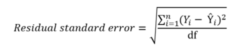
잔차표준오차 (RSE)
- RSE 는 실제 값이 추정한 회귀선으로부터 얼마나 벗어날지에 대한 평균값을 의미한다.
- residVar = sumSqrResids / (n - 2)
X = x[:,np.newaxis] # manipulate shape to row/col fmt
yPredict = Fmodel.predict(X) # predict y for x
resids = y - yPredict # series with delta between actual and predicted  # 실제값 - 예측값

sumSqrResids = np.square(resids).sum()  # 잔차 제곱합
n = len(X)
residVar = sumSqrResids / (n -2)
residSD = np.sqrt(residVar)
print("Residuals Standard Deviation:", residSD.round(2))

plt.scatter(x,resids)  # 아버지 키 - 잔차 그래프
plt.axhline(y=0, color = "dimgrey")
plt.axhline(y=2*residSD, color = "dimgrey", linestyle='--' )
plt.axhline(y=-2*residSD, color = "dimgrey", linestyle='--' )
plt.show()
Residuals Standard Deviation : 3.45

3) Determining the R-Squared Value

rSquared = sum(np.square(yPredict - df['Height'].mean())) / sum(np.square(df['Height'] - df['Height'].mean()))
print(rSquared.round(3))   # 결정계수 : 0.076
7. Centering and Normalising Data
- Centering Data
- 앞서 어머니의 키와 아버지의 키를 비교했을 때 아버지의 키가 어머니의 키보다 더 큰 값을 가졌다.
- 따라서 더 쉽게 비교하기 위해서 중심화를 시켜주어야 한다.
- 원래값에서 평균값을 제거한 후 선형회귀에 적합시킨다.
fatherCentered = df['Father'] - np.mean(df['Father'])
motherCentered = df['Mother'] - np.mean(df['Mother'])
childCentered = df['Height'] - np.mean(df['Height'])

Fmodel.fit(fatherCentered.values.reshape(-1,1),childCentered)   # Fmodel = LinearRegression(fit_intercept=True)  # 선형회귀 모형
print('(Height on Father) Coefficient: ', Fmodel.coef_)
print('Intercept: ', Fmodel.intercept_, '\n')

Mmodel.fit(motherCentered.values.reshape(-1,1),childCentered)
print('(Height on Mother) Coefficient: ', Mmodel.coef_)
print('Intercept: ', Mmodel.intercept_)
(Height on Father) Coefficient: [0.39938127] Intercept: 4.9365959103391907e-14
(Height on Mother) Coefficient: [0.31317952] Intercept: 6.806597041868856e-14
- 아버지 키와 자식 키의 선형회귀 적합 결과 y = intercept + 0.4 x
- 어머니 키와 자식 키의 선형회귀 적합 결과 y = intercept + 0.3 x_2

fatherCentered.values.shape   # (898,)
fatherCentered.values.reshape(-1,1).shape  # (898, 1)
중심화 시킨 후의 산점도와 회귀 직선 그래프


- 센터링 전과 후의 그래프를 비교해보면, 센터링된 데이터가 비교하기 수월하다.
- Normalising the Data
데이터를 표준편차로 나누어 정규화를 시켜주었다.
Zf = fatherCentered / np.std(fatherCentered)
Zm = motherCentered / np.std(motherCentered)
Zy = childCentered / np.std(childCentered)

print("Centered father data Std Dev:", np.std(Zf))  # 정규화시킨것의 표준편차
print("Centered mother data Std Dev:", np.std(Zm))
print("Centered child data Std Dev:", np.std(Zy))
Centered father data Std Dev: 1.0000000000000004
Centered mother data Std Dev: 0.9999999999999991
Centered child data Std Dev: 0.9999999999999978
정규화된 데이터로 선형회귀 적합
# 정규화된 데이터로 선형회귀 적합
Fmodel.fit(Zf.values.reshape(-1,1),Zy)
Mmodel.fit(Zm.values.reshape(-1,1),Zy)

xpredNorm = np.linspace(-5, 5).reshape(-1,1)
Fpred = Fmodel.predict(xpredNorm)
Mpred = Mmodel.predict(xpredNorm)

plt.scatter(Zf,Zy)
plt.scatter(Zm,Zy)

plt.plot(xpredNorm,Fpred)
plt.plot(xpredNorm,Mpred)

plt.legend(["father", "mother"])

plt.show()

1.2.2 Solving interactive problems with reinforcement learning
Another type of machine learning is reinforcement learning 강화 학습. In reinforcement learning, the goal is to develop a system (agent) that improves its performance based on interactions with the environment.
Since the information about the current state of the environment typically also includes a so-called reward signal 보상 신호, we can think of reinforcement learning as a field related to supervised learning.
However, in reinforcement learning this feedback is not the correct ground truth label or value, but a measure of how well the action was measured by a reward function. Through its interaction with the environment, an agent can then use reinforcement learning to learn a series of actions that maximizes this reward via an exploratory trial-and-error approach or deliberative planning.
A popular example of reinforcement learning is a chess engine. Here, the agent decides upon a series of moves depending on the state of the board (the environment), and the reward can be defined as win or lose at the end of the game:
또 다른 유형의 머신러닝은 강화 학습 입니다. 강화학습은 환경과의 상호작용을 바탕으로 성능을 향상시키는 시스템(agent)을 개발하는 것이 목표다.
환경의 현재 상태에 대한 정보에는 일반적으로 소위 보상 신호도 포함되어 있기 때문에 강화 학습은 지도 학습과 관련된 분야라고 생각할 수 있습니다.
그러나 강화 학습에서 이 피드백은 올바른 지상 True 라벨이나 값이 아니라 보상 함수에 의해 조치가 얼마나 잘 측정되었는지에 대한 척도이다. 그런 다음 환경과의 상호 작용을 통해 에이전트는 강화 학습을 사용하여 탐색적 시행착오 접근법 또는 숙고적 계획을 통해 이러한 보상을 최대화하는 일련의 조치를 학습할 수 있다.
강화 학습의 인기 있는 예는 체스 엔진이다. 여기서 에이전트는 보드의 상태(환경)에 따라 일련의 움직임을 결정하며, 보상은 게임이 끝날 때 승패라고 정의할 수 있다.

There are many different subtypes of reinforcement learning. However, a general scheme is that the agent in reinforcement learning tries to maximize the reward by a series of interactions with the environment.
Each state can be associated with a positive or negative reward, and a reward can be defined as accomplishing an overall goal, such as winning or losing a game of chess. For instance, in chess the outcome of each move can be thought of as a different state of the environment. To explore the chess example further, let's think of visiting certain locations on the chess board as being associated with a positive event—for instance, removing an opponent's chess piece from the board or threatening the queen. Other positions,
however, are associated with a negative event, such as losing a chess piece to the opponent in the following turn.
Now, not every turn results in the removal of a chess piece, and reinforcement learning is concerned with learning the series of steps by maximizing a reward based on immediate and delayed feedback.
강화 학습에는 다양한 하위 유형이 있습니다. 그러나 일반적인 계획은 강화 학습의 에이전트가 환경과의 일련의 상호 작용을 통해 보상을 최대화하려고 하는 것이다.
각 상태는 긍정적이거나 부정적인 보상과 연관될 수 있으며, 보상은 체스 게임의 승패와 같은 전반적인 목표를 달성하는 것으로 정의될 수 있다. 예를 들어 체스에서는 각 동작의 결과가 환경의 다른 상태로 생각될 수 있다. 체스 예제를 자세히 살펴보려면 체스 보드의 특정 위치를 방문하는 것이 긍정적인 이벤트(예: 보드에서 상대방의 체스 말을 제거하거나 퀸을 위협하는 경우)와 관련이 있다고 생각해 보겠습니다.
그러나 다른 포지션들은 다음 차례에서 체스 피스를 상대방에게 지는 것과 같은 부정적인 이벤트와 관련이 있다.
이제, 모든 차례가 체스 피스의 제거로 이어지는 것은 아니며, 강화 학습은 즉각적이고 지연된 피드백을 기반으로 보상을 최대화함으로써 일련의 단계를 학습하는 것과 관련이 있다.
주어진Environment 에서 Agent 가 더 높은 Reward 를 위해 최적의 Action 을 취해나가는 학습 과정
예 : 자전거를 배우는 어린아이
- Agent : 어린아이
- environment : 학교 운동장
- Action : 핸들을 이리저리 흔들면서 노력함
- Reward : 넘어지지 않고 지속된 시간이 길어짐
1.2.3 Discovering hidden structures with unsupervised learning
- 비지도학습의 클러스터링
- 비지도학습의 차원축소
In supervised learning, we know the right answer beforehand when we train our model, and in reinforcement learning, we define a measure of reward for particular actions by the agent. In unsupervised learning,
however, we are dealing with unlabeled data or data of unknown structure. Using unsupervised learning techniques, we are able to explore the structure of our data to extract meaningful information without the guidance of a known outcome variable or reward function.
지도 학습에서는 모델을 훈련할 때 정답을 미리 알고 강화 학습에서는 에이전트의 특정 행동에 대한 보상 척도를 정의합니다.
그러나 비지도 학습에서는 레이블이 없는 데이터 또는 알려지지 않은 구조의 데이터를 다루고 있다. 비지도 학습 기술을 사용하여 알려진 결과 변수 또는 보상 함수의 안내 없이 의미 있는 정보를 추출하기 위해 데이터 구조를 탐색할 수 있다.
1) Finding subgroups with clustering
Clustering 군집, 집락 is an exploratory data analysis technique that allows us to organize a pile of information into meaningful subgroups (clusters) without having any prior knowledge of their group memberships.
Each cluster that arises during the analysis defines a group of objects that share a certain degree of similarity but are more dissimilar to objects in other clusters, which is why clustering is also sometimes called unsupervised classification 비지도 분류.
Clustering is a great technique for structuring information and deriving meaningful relationships from data.
For example, it allows marketers to discover customer groups based on their interests, in order to develop distinct marketing programs.
The following figure illustrates how clustering can be applied to organizing unlabeled data into three distinct groups based on the similarity of their features x_1 and x_2:
클러스터링은 그룹 구성원에 대한 사전 지식 없이도 의미 있는 하위 그룹(클러스터)으로 정보 더미를 구성할 수 있는 탐색적 데이터 분석 기법이다.
분석 중에 발생하는 각 클러스터는 일정 정도의 유사성을 공유하지만 다른 클러스터에 있는 개체와 더 다른 개체 그룹을 정의하므로 클러스터링을 비지도 분류라고도 합니다.
클러스터링은 정보를 구조화하고 데이터에서 의미 있는 관계를 도출하기 위한 훌륭한 기술이다. 예를 들어, 그것은 마케터들이 뚜렷한 마케팅 프로그램을 개발하기 위해 그들의 관심사에 따라 고객 그룹을 발견할 수 있게 한다.다음 그림은 레이블이 지정되지 않은 데이터를 특징 x_1과 x_2의 유사성에 따라 세 개의 다른 그룹으로 구성하는 데 클러스터링을 적용하는 방법을 보여줍니다.

2) Dimensionality reduction for data compression
Another subfield of unsupervised learning is dimensionality reduction 차원축소.
Often we are working with data of high dimensionality—each observation comes with a high number of measurements—that can present a challenge for limited storage space and the computational performance of machine learning algorithms.
Unsupervised dimensionality reduction is a commonly used approach in feature preprocessing to remove noise from data, which can also degrade the predictive performance of certain algorithms, and compress the data onto a smaller dimensional subspace while retaining most of the relevant information.
Sometimes, dimensionality reduction can also be useful for visualizing data, for example, a high-dimensional feature set can be projected onto one-, two-, or three-dimensional feature spaces in order to visualize it via 3D or 2D scatterplots or histograms. The following figure shows an example where nonlinear dimensionality reduction was applied to compress a 3D Swiss Roll onto a new 2D feature subspace:
비지도 학습의 또 다른 하위 분야는 차원 축소이다.
우리는 종종 제한된 스토리지 공간에 문제가 될 수 있는 높은 차원의 데이터(각 관측치마다 측정 횟수가 많음)를 연구하고 있습니다. 그리고 기계 학습 알고리즘의 연산 성능.
비지도 치수 감소는 특정 알고리즘의 예측 성능을 저하시킬 수 있는 데이터의 노이즈를 제거하고 대부분의 관련 정보를 유지하면서 데이터를 더 작은 치수 하위 공간으로 압축하기 위해 기능 전처리에서 일반적으로 사용되는 접근법이다.
때때로 치수 감소는 데이터를 시각화하는 데 유용할 수 있다. 예를 들어, 3D 또는 2D 산점도 또는 히스토그램을 통해 시각화하기 위해 고차원 형상 세트를 1차원, 2차원 또는 3차원 형상 공간에 투영할 수 있다. 다음 그림은 비선형 치수 감소를 적용하여 3D 스위스 롤을 새로운 2D 피쳐 하위 공간으로 압축한 예를 보여 줍니다.

참고
- 머싱러닝에서는 입력 데이터의 각 특성을 하나의 축으로 생각하여 벡터 공간 (vector space)이라는 표현을 사용함. 특성을 줄여 차원이 낮아진 데이터를 부분 공간 (sub-space)이라고 표현함
- 스위스롤 (Swiss roll, 롤 레이크 Roll cake): 크림이나 잼을 넣어 둘둘 말은 형태의 케이크
semi-supervised learning 준지도 학습 and self-supervised learning 자기주도 학습
- 준지도 학습: 레이블이 있는 데이터셋과 레이블이 없는 데이터셋을 모두 사용함
- 자기주도 학습: 입력이 타깃이 되는 지도 학습 (예) autoencoder 오토인코더
1.3 Introduction to the basic terminology and notations
- sample 표본 instance 인스턴스 observation 관측값
- feature 특징, 특성 attribute 속성 measurement 측정 dimension 차원
To keep the notation and implementation simple yet efficient, we will make use of some of the basics of linear algebra.
In the following chapters, we will use a matrix and vector notation to refer to our data.
We will follow the common convention to represent each sample as a separate row in a feature matrix X, where each feature is stored as a separate column.
표기법과 구현을 단순하면서도 효율적으로 유지하기 위해 선형 대수의 몇 가지 기본을 활용할 것이다.
다음 장에서는 데이터를 참조하기 위해 행렬과 벡터 표기법을 사용할 것입니다.
일반적인 관례에 따라 각 표본을 feature matrix X에서 개별행으로 나타내며, 여기서 각 feature은 별도의 열로 저장된다.
iris 데이터셋 시각화
from sklearn.datasets import load_iris
from matplotlib import pyplot as plt
import seaborn as sns
import numpy as np
import pandas as pd

from IPython.display import Image
# dataset 'iris'를 array로 불러오기
Iris = load_iris()
Iris


# np_r: 배열을 왼쪽에서 오른쪽으로 붙이기
# np.c_: 배열을 위에서 아래로 붙이기

Iris_data = pd.DataFrame(data = np.c_[Iris['data'], Iris['target']], columns = Iris['feature_names'] + ['target'])
Iris_data

# features 만 추출함
X_data = Iris_data.iloc[:,:-1]
X_data


# target 만 추출함
Y_data = Iris_data.iloc[:,[-1]]
Y_data


seaborn.pairplot
참고 : https://seaborn.pydata.org/generated/seaborn.pairplot.html
# dataset 'iris'를 array로 불러오기
#Iris = load_iris()

# daraset 'iris'를 DataFrame으로 바로 불러오기
iris = sns.load_dataset("iris")
iris

iris = sns.load_dataset("iris")
g = sns.pairplot(iris)
# Use kernel density estimates for univariate plots.
g = sns.pairplot(iris, diag_kind="kde") # 커널밀도함수


# different levels of a categorical variable by the color of plot elements
g = sns.pairplot(iris, hue = "species")
색상을 다르게 지정
# different color palette
g = sns.pairplot(iris , hue ="species", palette="husl")
마커를 다르게 지정
# different markers
g = sns.pairplot(iris, hue="species", markers=["o","s","D"])
점의 테두리 설정 + 음영효과
g = sns.pairplot(iris, diag_kind="kde",markers="o",
                plot_kws=dict(s=50,edgecolor="b",linewidth=1), # kws : 점의 속성 변경
                diag_kws=dict(shade=True),hue="species")  # # shade=True 음영효과 설정
두 개의 변수로 산점도 그리기
# a subset of variables
g = sns.pairplot(iris, vars=["sepal_width", "sepal_length"])
g = sns.pairplot(iris, vars=["sepal_width", "sepal_length"], hue = "species")

그래프 크기 지정
# larger plots
g = sns.pairplot(iris, height=5,
                 vars=["sepal_width", "sepal_length"])
# larger plots
g = sns.pairplot(iris, height=5,
                vars=["sepal_width","sepal_length"],hue = "species")
네 개의 변수로 산점도 그리기
# different variables in the rows and columns
g = sns.pairplot(iris,
                x_vars=["sepal_width","sepal_length"],
                y_vars=["petal_width","petal_length"])
# different variables in the rows and columns
g = sns.pairplot(iris,
x_vars=["sepal_width", "sepal_length"],
y_vars=["petal_width", "petal_length"], hue = "species")

산점도 아래쪽만 나타내기
# Plot only the lower triangle of bivariate axes.
g = sns.pairplot(iris, corner=True)
산점도 그림에 회귀선 추가하기
# Fit linear regression models to the scatter plots.
g = sns.pairplot(iris, kind="reg")
# Fit linear regression models to the scatter plots.
g = sns.pairplot(iris, kind="reg", hue="species")

커널 밀도함수 그래프
g = sns.PairGrid(iris)
g.map_diag(sns.kdeplot)  # 대각선 그래프 : 커널밀도함수 그래프
g.map_offdiag(sns.kdeplot, n_level=6)
sns.pairplot(iris, kind="kde")


seaborn.jointplot
참고 : https://seaborn.pydata.org/generated/seaborn.jointplot.html
산점도와 히스토그램을 같이 그리기
# Draw a scatterplot with marginal histograms.
g = sns.jointplot(x="petal_length",y="petal_width",data=iris)
# Add regression and kernel density fits.
g = sns.jointplot("petal_length","petal_width",data= iris, kind="reg")


Hexbon plot 와 같이 그리기
+ 색상표 참고

# Replace the scatterplot with a joint histogram using hexagonal bins.
g = sns.jointplot("petal_length","petal_width",data=iris, kind="hex")
with sns.axes_style("white"):
sns.jointplot(x="petal_length",y="petal_width",data=iris,kind="hex",color="k")

with sns.axes_style("dark"):
    sns.jointplot(x="petal_length",y="petal_width",data=iris,kind="hex",color="c")
커널 밀도함수와 같이 그리기
sns.jointplot(x="petal_length",y="petal_width",data=iris, kind="kde",shade=True)f , ax = plt.subplots(figsize=(6,6))
sns.kdeplot(iris.petal_length,iris.petal_width, ax=ax)
sns.rugplot(iris.petal_length, color="g", ax=ax)
sns.rugplot(iris.petal_width,vertical=True, ax=ax)

f, ax = plt.subplots(figsize=(6,6))
cmap = sns.cubehelix_palette(as_cmap=True, dark=0, light=1, reverse=True)
sns.kdeplot(iris.petal_length,iris.petal_width,cmap=cmap, n_levels=60, shade=True)
f, ax = plt.subplots(figsize=(6,6))
cmap = sns.cubehelix_palette(as_cmap=True, dark=0, light=3, reverse=True)
sns.kdeplot(iris.petal_length,iris.petal_width,cmap=cmap, n_levels=60, shade=True)

f, ax = plt.subplots(figsize=(6,6))
cmap = sns.cubehelix_palette(as_cmap=True, dark=0, light=1, reverse=True)
sns.kdeplot(iris.petal_length,iris.petal_width,cmap=cmap, n_levels=60, shade=False)
g = sns.jointplot(x="petal_length",y="petal_width",data=iris,kind="kde",color="m",shade=True)
g.plot_joint(plt.scatter, c="w",s=30,linewidth=1,marker="+")
g.ax_joint.collections[0].set_alpha(0)
g.set_axis_labels("$X$","$Y$")

seaborn.boxplot
참고 : https://seaborn.pydata.org/generated/seaborn.boxplot.html
ax = sns.boxplot(x="species",y="sepal_length",data=iris)
seaborn.violinplot
참고 : https://seaborn.pydata.org/generated/seaborn.violinplot.html
ax = sns.violinplot(x="species",y="sepal_length",data=iris)
Visualizing the distribution of a dataset
참고 : https://seaborn.pydata.org/tutorial/distributions.html
x = iris["sepal_length"]
sns.displot(x)
x = iris["sepal_length"]
sns.displot(x,kde=True)

sns.distplot(x, kde=True, rug=True)sns.distplot(x, hist=False, rug=True)sns.kdeplot(x, shade=True)


1.4 A roadmap for building machine learning systems

1.4.1 Preprocessing - getting data into shape
Let's begin with discussing the roadmap for building machine learning systems.
Raw data rarely comes in the form and shape that is necessary for the optimal performance of a learning algorithm.
Thus, the preprocessing of the data is one of the most crucial steps in any machine learning application. If we take the Iris flower dataset from the previous section as an example, we can think of the raw data as a series of flower images from which we want to extract meaningful features.
Useful features could be the color, the hue, the intensity of the flowers, the height, and the flower lengths and widths.Many machine learning algorithms also require that the selected features are on the same scale for optimal performance, which is often achieved by transforming the features in the range [0, 1] or a standard normal distribution with zero mean and unit variance, as we will see in later chapters.
Some of the selected features may be highly correlated and therefore redundant to a certain degree. In those cases, dimensionality reduction techniques are useful for compressing the features onto a lower dimensional subspace. Reducing the dimensionality of our feature space has the advantage that less storage space is required, and the learning algorithm can run much faster. In certain cases, dimensionality reduction can also improve the predictive performance of a model if the dataset contains a large number of irrelevant features (or noise), that is, if the dataset has a low signal-to-noise ratio.
To determine whether our machine learning algorithm not only performs well on the training set but also generalizes well to new data, we also want to randomly divide the dataset into a separate training and test set.
We use the training set to train and optimize our machine learning model, while we keep the test set until the very end to evaluate the final model.
1.4.2 Training and selecting a predictive model
As we will see in later chapters, many different machine learning algorithms have been developed to solve different problem tasks. An important point that can be summarized from David Wolpert's famous No free lunch theorems '공짜 점심 없음' 이론 is that we can't get learning "for free" (The Lack of A Priori Distinctions Between Learning Algorithms, D.H. Wolpert 1996; No free lunch theorems for optimization, D.H. Wolpert and W.G. Macready, 1997).
Intuitively, we can relate this concept to the popular saying, I suppose it is tempting, if the only tool you have is a hammer, to treat everything as if it were a nail (Abraham Maslow, 1966). For example, each classification algorithm has its inherent biases, and no single classification model enjoys superiority if we don't make any assumptions about the task.
In practice, it is therefore essential to compare at least a handful of different algorithms in order to train and select the best performing model.
But before we can compare different models, we first have to decide upon a metric to measure performance 성능 측정 지표. One commonly used metric is classification accuracy 분류 정확도, which is defined as the proportion of correctly classified instances.
One legitimate question to ask is this: how do we know which model performs well on the final test dataset and real-world data if we don't use this test set for the model selection, but keep it for the final model evaluation? In order to address the issue embedded in this question, different cross-validation 교차타당성 techniques can be used where the training dataset is further divided into training and validation subsets in order to estimate the generalization performance of the model.
Finally, we also cannot expect that the default parameters of the different learning algorithms provided by software libraries are optimal for our specific problem task. Therefore, we will make frequent use of hyperparameter 초매개변수 optimization techniques that help us to fine-tune the performance of our model in later chapters.
Intuitively, we can think of those hyperparameters as parameters that are not learned from the data but represent the knobs of a model that we can turn to improve its performance. This will become much clearer in later chapters when we see actual examples.

1.4.3 Evaluating models and predicting unseen data instances
After we have selected a model that has been fitted on the training dataset, we can use the test dataset to estimate how well it performs on this unseen data to estimate the generalization error. If we are satisfied with its performance, we can now use this model to predict new, future data. It is important to note that the parameters for the previously mentioned procedures, such as feature scaling and dimensionality reduction, are solely obtained from the training dataset, and the same parameters are later reapplied to transform the test dataset, as well as any new data samples—the performance measured on the test data may be overly optimistic otherwise.
교육 데이터 세트에 적합한 모델을 선택한 후 테스트 데이터 세트를 사용하여 보이지 않는 이 데이터에서 얼마나 잘 수행되는지 추정하여 일반화 오류를 추정할 수 있다. 성능이 만족스러우면 이제 이 모델을 사용하여 새로운 미래 데이터를 예측할 수 있습니다. feature 스케일링 및 차원 축소와 같은 앞서 언급한 절차의 매개 변수는 교육 데이터 집합에서만 얻을 수 있으며, 나중에 동일한 매개 변수를 테스트 데이터 집합과 새로운 데이터 샘플을 변환하기 위해 다시 적용할 수 있습니다.
1.5 Using Python for machine learning
Python is one of the most popular programming languages for data science and therefore enjoys a large number of useful add-on libraries developed by its great developer and and open-source community.
Although the performance of interpreted languages, such as Python, for computation-intensive tasks is inferior to lower-level programming languages, extension libraries such as NumPy and SciPy have been developed that build upon lower-layer Fortran and C implementations for fast and vectorized operations on multidimensional arrays.
For machine learning programming tasks, we will mostly refer to the scikit-learn library, which is currently one of the most popular and accessible open source machine learning libraries.
1.6 Summary
In this chapter, we explored machine learning at a very high level and familiarized ourselves with the big picture and major concepts that we are going to explore in the following chapters in more detail. We learned that supervised learning is composed of two important subfields: classification and regression.
While classification models allow us to categorize objects into known classes, we can use regression analysis to predict the continuous outcomes of target variables.
Unsupervised learning not only offers useful techniques for discovering structures in unlabeled data, but it can also be useful for data compression in feature preprocessing steps. We briefly went over the typical roadmap for applying machine learning to problem tasks, which we will use as a foundation for deeper discussions and hands-on examples in the following chapters. Eventually, we set up our Python environment and installed and updated the required packages to get ready to see machine learning in action.
Later in this book, in addition to machine learning itself, we will also introduce different techniques to preprocess our dataset, which will help us to get the best performance out of different machine learning algorithms. While we will cover classification algorithms quite extensively throughout the book, we will also explore different techniques for regression analysis and clustering.
We have an exciting journey ahead, covering many powerful techniques in the vast field of machine learning.
However, we will approach machine learning one step at a time, building upon our knowledge gradually throughout the chapters of this book. In the following chapter, we will start this journey by implementing one of the earliest machine learning algorithms for classification, which will prepare us for Chapter 3, A Tour of Machine Learning Classifiers Using scikit-learn, where we cover more advanced machine learning algorithms using the scikit-learn open source machine learning library.
'파이썬 > 머신러닝,딥러닝' 카테고리의 다른 글
| 모델 복잡도 제한을 위한 L1 , L2 규제 (0) | 2022.04.14 |
|---|---|
| Confusion matrix - Iris 데이터를 이용한 퍼셉트론 훈련 (0) | 2022.03.31 |
| 텐서플로우를 이용한 신경망 구현 예제 (0) | 2022.03.29 |
| K-Fold Cross Validation 와 validation 데이터에 대한 이해 (0) | 2022.03.17 |
| Bagging - for 문을 이용하여 Bagging 구현 (0) | 2022.01.27 |


